In the previous sections, we learned how to train Flow Matching, or a spreadsheet model, to sample from a distribution. This is a general formula that can be applied to a wide variety of data types and applications.
In this section, we explore specific instances of large-scale image and video generation, including well-known models such as FLUX 2.0, Stable Diffusion 3, Nano Banana and VEO-3 or Meta Movie Gen Video.
Finally, we will apply what we have learned in experimental lessons to build our own version from scratch.
Neural network architectureWe first discussed how to convert the original input (including time and boot variables, i.e. discrete labels or original text) to the original input (including time and boot variables).EmbeddedThe popular architectural options discussed later, including the U-Net and the diffusion transformer.
In spaceWe discussed:Variable from the encoderIt allows generative modeling in low-dimensional space, thus achieving ultra-high-resolution image generation.
Case studiesFinally, we take a closer look at the two most advanced image and video models mentioned above: Stable Diffusion 3 and Meta MovieGen.
6.1 Neural network architecture
Let's first turn our attention to the design of scalable neural network architectures for image-like models (such as images and videos).
Specifically, we'll explore how to implement a guided vector field in practice, whose parameters are: note that neural networks must have three inputs: a vector, a condition variable, a time value, and an output.
For low-dimensional distributions (e.g. toy distributions as seen in the previous sections), a multi-layered sensor (MLP, i.e. all-connected network) is sufficient to parameterize.
In other words, in this simple setup, forward propagation is sending the input into the MLP after it is pasted.
However, for complex high-dimensional distributions, such as images, video, and proteins, MLP may not be enough.
In the rest of this section, we consider the situation in the images and promote them to video.
First of all, we're going to look at the raw conditions of information about the cooking time and the condition variables of how cooking is done.EmbeddedThe vector value forms that can be processed for the model. Next, we discuss two common architectural options for this model:U-Netanddiffusion transformer(DiT)。
6.1.1 Embedded condition variables
Embedded timeFor a simple toy model, adding the original value to the input is enough to train a network to perform reasonably.Fourier characteristicsEmbedded into higher dimensional space, the model can more faithfully capture high frequency time dependence.
The frequency is set as:
The choice of this type of TimeEmb is standard practice, but this precise form is not strictly necessary.
Embedded category tagsWhen it comes to just a class tag, the simplest approach is usually to learn an embedded vector for each possible value directly and set it to that embedded vector. We would like to see these embedded parameters included in the parameters and learn them in training.
Embedded text inputThe method relies primarily on a frozen pre-training model. This model can be trained to map discrete text inputs into a continuous vector to capture relevant information.CLIP(Contrastive Language-Image Pre-training)。
CLIP is trained to learn a shared embedded space between images and text prompts, with training losses designed to bring image embeddings closer to their corresponding prompts while removing the embeddings from other images and prompts.
In some cases, it may not be possible to compress the entire sequence into a single representation. In this case, an additional pre-training transformer can be used to embed the prompt to obtain the embedded sequence. It is also common for conditioning to combine multiple such pre-training embeddings to take advantage of each model at the same time. For our purposes, we can simply assume that the post-embedded shape of the application prompt is as follows:
6.1.2 Diffusion Transformer
Before getting into the details of these architectures, let's take a look at the description of the image in the introduction: the image is essentially a vector. Here it shows the number of channels (RGB images usually have a color channel) and the height and width of the image (in pixels) respectively.diffusion transformer(DiT)With their variants, they use attention mechanisms to construct networks. Diffusion transformers come in different genres. Here we explain a general design and pay attention to specific implementations that may differ depending on model and application.
In the remainder of this section, we use the hidden dimension, the number of transformer layers, and the prime number of each layer.
The diffusion transformer is based on:vision transformer(ViT)Its main idea was essentially to cut an image into patches, embed these patches to obtain a sequence of tokens, and then process the token through standard attention. Finally, an anti-patchify operation was applied at the end to restore the correct shape of the image. The initial patchify operation simply rearranged the image volume to:
Then we apply a linear transformation to the output and get the final patch embedded:
Among them is the input of a learning weight matrix, diffusion transformer, and then time embedding, prompt embedding, and patch image volumes (see section 6.1.1):
Note that all elements now have the required hidden dimensions of the transformer. The diffusion transformer is then updated through the transformer layer in DiTBlock (see note 29 for details):
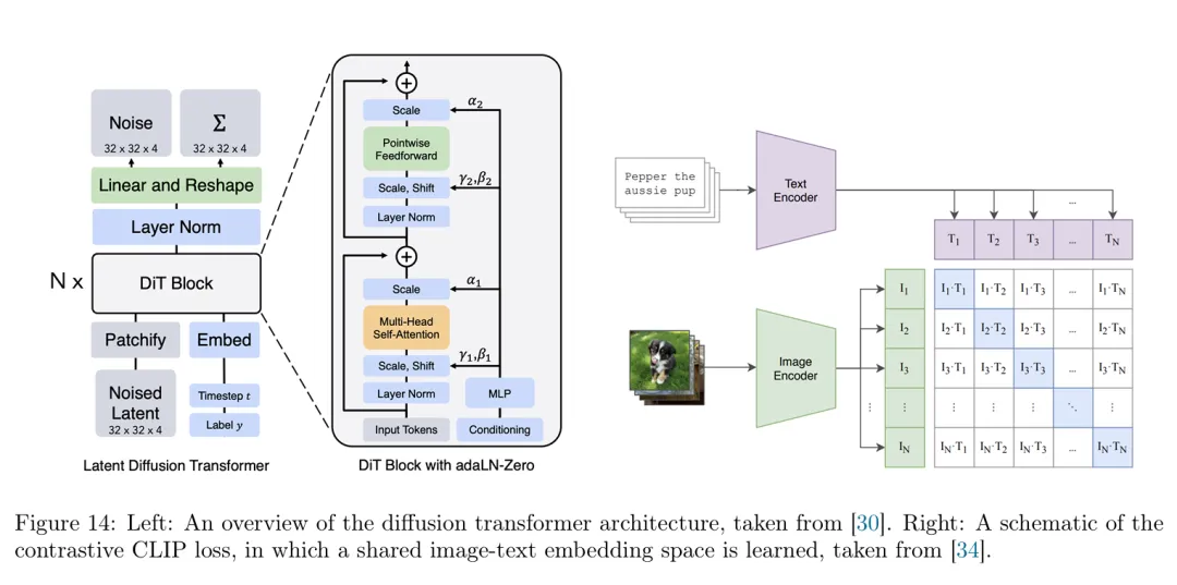
Figure 14: Left: diffusion transformer architecture overview. Right: diagram of CLIP loss in shared image-text embedded space.
Finally, one final operation imposes an anti-patchify operation to map the DiT output back to the expected output shape:
The final voltage is then used as the output and predicted speed of the model.
It's the first time I've ever heard of this.
For the sake of completeness, we give a brief mathematical description of a single layer of DiT. Although we try to contain enough detail to understand the DiT model family, readers should note that the DiT model family emphasizes algorithmic selection rather than architectural details.
The current sequence of patch tokens is displayed here, and the embedded boot variable is displayed here, and then a typical DiT block is updated with (i) self-attention on the patch, (ii) cross-attention to the prompt, and (iii) time conditions for AdaLN self-alignment.
Concentrating attentionIt's a question, it's a key, it's a value
In this case, the softmax is applied according to the rules.
Multi-headed attentionIn order to represent the number of heads, represent the dimensions of each head, learn the projection matrix for each head.
The source sequence is either
Spell out the heads and project the output:
Time conditioning by self-adaptation to unificationA standard option in DiT is to generate a channel-by-channel scaling/deviation parameter to activate modulation into unification. Specifically, order for an MLP and set
In which (or depending on the implementation, is a pair of different sub-layers such as attention and MLP) a given token matrix and a convergence algorithm (such as LayerNorm) define convergence.
It shows the exponential multiplication of the elements broadcast in the token dimension.
Integrating togetherDiTBlock is a combination of the following functions:
Where MLP is a position-by-position frontend network, it is a door control parameter that can be learned. The output becomes the next in the patch-token sequence. Finally, we note that DiT is typically simpler, such as the type of condition implemented in experimental classes, which tends to use time and class-based AdaNorm conditioning instead of the cross-attention layer.
6.1.3 U-Net
U-NetThe architecture is an alternative to the DiT architecture, which is a specific type of convolutional neural network. Initially designed for image splitting, its key characteristic was that both inputs and outputs have image shapes (possibly with different number of channels). This makes it very suitable for parametric vector fields, since its input shape is an image and its output shape is an image at fixed times.
U-Net is made up of a seriesCodifierand a series of correspondingThe decoderThere's one in the middle, we call it.midcoderFor the sake of convenience, let's go through the path of the image (we take) through the U-Net:
Note that when we pass an image through the encoder, the number of channels increases, while the height and width of the image decreases. The encoder and encoder are usually composed of a series of convolutional layers (activation functions, clustering operations, etc.).
Two points not shown above: first, input is often sent to an initial pre-encoded block in order to increase the number of channels before the first encoder block is sent. Second, between the encoder and the encoder is usually passed.Poor connectivityConnected.
At a higher level, most U-Net involve some of the variants described above. However, some design choices may vary in practice depending on implementation. In particular, a common feature of pure-volume architectures is that the attention layer is added throughout the encoder and encoder. U-Net is named for its "U" stack (see Figure 15).
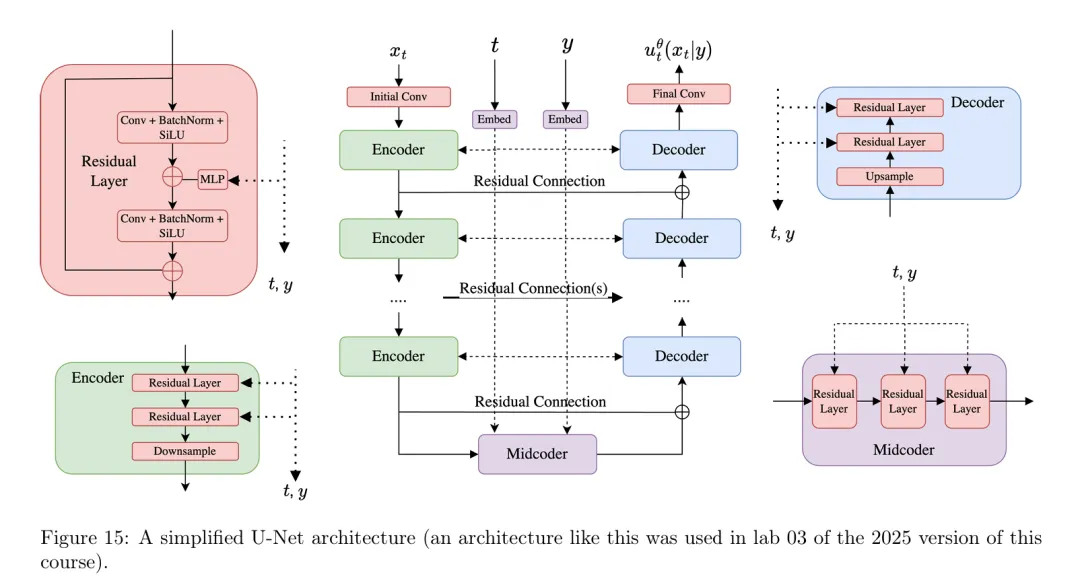
Figure 15: A simplified U-Net architecture (similar architecture used in experimental class 03 of the 2025 version of the course)
6.2 Working in Hidden Space: Differentiation from Coding
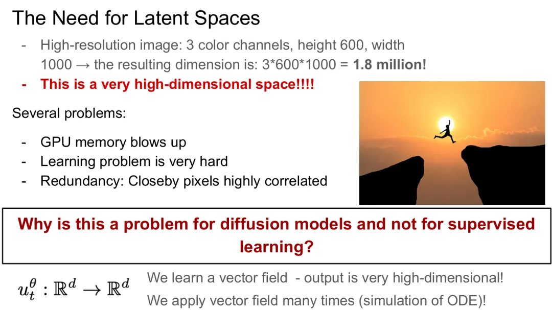
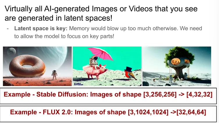
Until now, we've been operating in data space. However, as we expand models in this space to increasingly high-resolution images, the cost quickly becomes unspeakably high.
For example, an image of 1024×1024 with 3 RGB color channels corresponds to the total dimension. Note that this dimension increases as the number of pixels in the video increases. You can imagine that training in such a space quickly becomes impossible.
Unlike image classification, low-dimensional output does not allow for the reduction of volumes, and our flow modeling method requires the same output as the input size.
So the important question has become:How do we model high-dimensional images in a reasonable memory and computational budget?
6.2.1 Standards are encoded
The natural answer to this question is:CompressionFor example, the actual image space is located near a low-dimensional fluid in high-dimensional image space. More specifically, we can consider aCodifierand aThe decoderTogether, they map the original image as a hidden variable (and vice versa). Dimensions are usually selected to be much smaller.
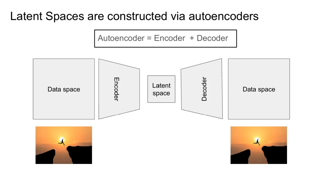
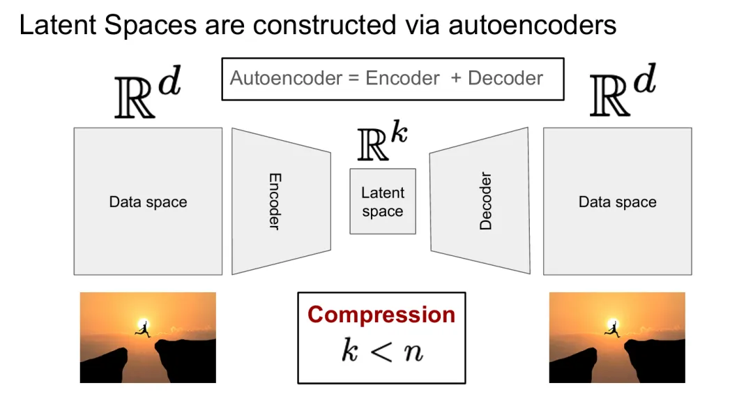
For images, for example, a common practice is to take samples, for example.Self-codingIdeally, and is chosen to achieve high rebuilding quality in the average sense, making it look like.Rebuilding lossesTraining:
It measures the square error between the original data point and the result of the reconstruction.
Applicability of generated modelingRegrettably, reconstruction losses alone are not enough to train a "good" self-encoder. In retrospect, our ultimate goal is to train a generating model in cache space and target a given cache distribution. A pair of generating models is achieved by decoding the output of the cache generating model through the decoder.
But as with the self-encoder we're currently building, one subtle problem is that we can't control it, so we can't guarantee it behaves well enough to train a generating model -- that's pretty, simple, class-wise.
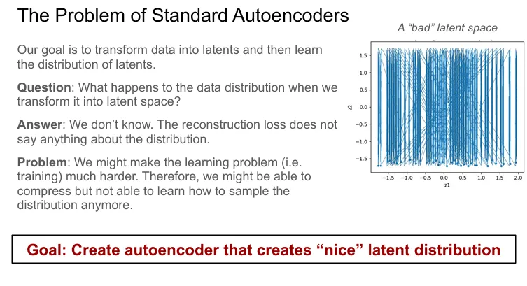
Although we have compressed the data into hidden space, it is possible to transform the data distribution into a distribution that is difficult to learn.
So the question is: how do we make sure that the hash distribution behaves well and is easy to learn? In order to allow for explicit rule masking of the hash distribution that will lead from the encoder to the more general framework of probability concepts, we then introduce the variable separation from the encoder.
6.2.2 Differentiation from encoder
Variable from the encoder (VAE)It is a constraint on the deterministic function by loosening the encoder and decoding the encoder, which is formalized by the encoder from the deterministic standard.
Specifically, consider an encoder with a parameter and a decoder with a parameter.
Here, as a neural network parameter, the diagram represents an opposite matrix. To encode or decode a variable, we take a sample.
Finally, note that once and for all, we restore the standard encoder itself. Let's look at how to reconstruct the loss.
Note the two changes: from the certainty coding to the random coding, which we are now sampling. In addition, we take the negative pairs of decoded multiples, i.e. losses, effectively asking: given all the possible decoding/coding, how many of our original data points are likely to be encoded and then decoded back?
In this case, we use the density of the normal distribution of Gauss (see equation 97). Thus, the difference between VAE reconstruction losses and standard AE reconstruction losses is that we have to consider all possible averages under coding.
Many implementations (including in experimental classes) take and learn the parametric constants (with and without) to avoid pathological behaviour and numerical instability during learning differences.
Therefore, the VAE reconstruction loss in this case is basically the standard decoder reconstruction loss plus the randomness and constancy of the encoding:
Now let's re-examine the goal: we want to create coding for the data distribution so that mapping to hidden space makes the distribution "beautiful" and easy to learn.
So now we're going to introduce a variable to the equation.Predetermined distributionFor our purposes, take as an all-round homosexual goose.
This selection of prior distributions effectively represents the "ideal" appearance of binary distributions. Normal distributions are easy to learn and therefore meet the goal of obtaining "trainable" binary distributions.
It's the same thing.In this case, it is not possible to calculate the distance between the two points.。
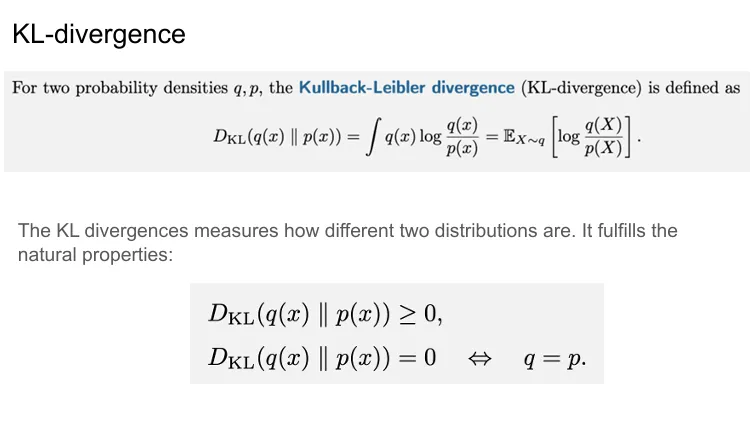
KL scattering is a basic method of measuring the difference in probability distribution between two probabilities. The detailed explanation is beyond the scope of this work, but we give a brief background as a reminder in note 30.
The loss defined in equation 75 is very intuitive: we want the encoded distribution to look like a Gaussian distribution. If we do that for all of them, nature expects our inherent distribution to look like a Gaussian distribution.
Note 30 ((KL scattered background)
It's the same thing with two probability densities.The Kullback-Leibler scatteringDefined as
KL scattering is a standard measure of the discrepancy between distributions. In particular, KL scattering satisfies the following useful properties:
That is, it is always non-negative, and is zero if and only if the two probability distributions overlap.
To define the loss function of the differential decoder, we can now use the parameter weight to combine the reconstruction loss and the previous loss.VAE training objectives:
The first of these forces the binomial variables to be efficiently decoded back to the data, and the second forces our binomial distribution to be closer to Gaussian. The parameters control the intensity of each. To make the loss more specific, we derive the KL scattering under Gaussian conditions:
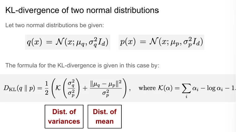
Example 31 ((KL scattering between each of the same geos)
For example, the Gaussian matrix for the inverse of the angles of a triangle, in which,
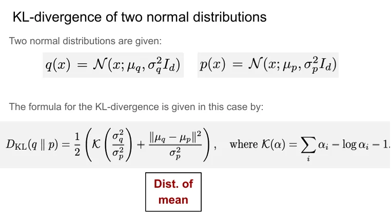
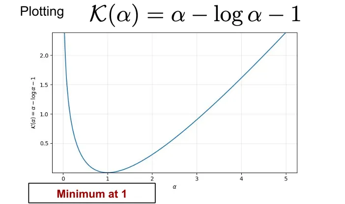
The above expression is intuitive. If the mean and the square of the variance overlap, it also increases the square error between the mean value vectors. Finally, the function has the only minimum value and is therefore the smallest at the time.
EvidenceThe density of the normal distribution for each dimension is given by the proof of the proof (see equation 97):
What is it?
Yes, it is.
And that's what we get.
The substitution equation (81) is equal to (80)..
Now suppose the encoder is Gauss-shaped.
This loss is intuitive: the mean value is punished for deviation from zero and the difference is punished for deviation from one.
All four of the above loss functions are very intuitive. The first is simply a reconstruction error. The second describes the uncertainty of the decoder: the smaller the gap, the more "confident" the decoder is, but also punishes reconstruction errors more severely.
VAE trainingThe remaining issue is discussing how to minimize VAE losses. The problem is that the expected distribution so far depends on the parameters themselves.Hard arithmetic techniquesI'm going to rewrite it.
We can take samples in the following ways:
Note that in this equation, the only noise/random source is that its distribution is unrelated.
After heavy parametrization, randomness only comes from, and its distribution does not depend on. Therefore, we can now minimize losses with standard deep learning tools.
For further simplification, we can set a constant everywhere and again get:
In Algorithm 6, we summarize the training process of VAE.
Practical NotesThe structure we developed above demonstrates the principles of encoder design. Of course, in practice, people may add more loss items or other constraints.
Selection (and KL warm-up)• Large forces the state of immobility closer to the original, but may damage the reconstruction and triggerConcentration testing(Coder ignores, output) A common method of stabilization isKL warm-upFrom the beginning, it gradually increased to the target value in the previous few epochs. However, among all modern self-encoders, it is very small, i.e.
The decoder is broken.Learn Gauss decoder differentials are numerically subtle, unless normalized, which can lead to decomposition. For stability, many implementations of fixed as a constant differential, which makes reconstruction losses and equilateral errors positive (except for constants).
Rebuilding losses beyond the pixel MSEFor images, the pixel-by-pixel Gaussian similarity (equivalent error) often results in too smooth reconstruction.Perceived Loss(Feature space loss) to improve concentration and reliability using pre-trained networks.
Combating mixed targets• To further enhance visual realism, it can be usedadversarial loss(VAE-GAN style) In conjunction with VAE targets, differentiators are used in decoding samples. This typically consolidates the output, but introduces additional optimization instability and additional hyperparameters.
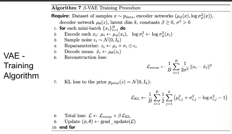
Algorithm 6- VAE training process (Fixed Differential Gaussian decoder)
Note 32 ((Working in outer space)
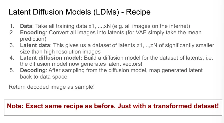
In order to train a latent generation model, we just have to follow the existing training formula, but we have to do it directly.In spaceIn training, we sample from the middle, including; in reasoning, we sample from the latent diffusion or flow model, and then decode with the decoder (note that we take average values rather than random samples to avoid noise distortion).
Intuitively, a well-trained self-encoder can be viewed as a filter for removing high frequency or other semantically meaningless details, so that the generated model is "focused" on important, perceptually relevant features.
At the time of writing this lecture, almost all of the most advanced methods of image and video generation follow the so-calledLatent diffusion paradigmThe flow or diffusion model is trained in the encoder's hidden space.
Importantly, however, people still need to train the self-encoder and then the spread model. Crucially, the performance now also depends on the self-encoder's ability to compress images to a hidden space and beautifully restore images.
We provide additional discussion on VAE in Appendix D.
6.3 Case studies: Stable Diffusion 3 and Meta Movie Gen
Finally, we briefly examine two mass-produced models to conclude this section: Stable Diffusion 3 for image generation and Meta Movie Gen Video for video generation.
As you will see, these models use the techniques that we have described in this work, and have additional architectural enhancements to accommodate both structured conditional models, such as text input.
6.3.1 Stable Diffusion 3
Stable Diffusion 3 is a series of state-of-the-art image generation models. These models were among the first to use large-scale latent diffusion models in image generation.
Stable Diffusion 3 uses the same conditions that we studied in this work for the Flow Matching goal (see Algorithm 4).
As outlined in their paper, they extensively tested various flow and dispersion alternatives and found that Flow Matching performed best. For training, it used a non-classifier to guide training.
In addition, Stable Diffusion 3 follows the methodology outlined in section 6.1, training in the latent space of the encoder.
To enhance text conditionality, Stable Diffusion 3 uses two different types of text embedments simultaneously: CLIP embedments, and sequence output generated by pre-trained instances of Google T5-XXL encoders. CLIP embedments provide roughness and coverage of the input text, while T5 embedments provide more fine-grained conditionality, allowing models to close specific elements of the order book.
In order to accommodate these sequence embedments, the authors proposed expanding the diffusion transformer to attend to image patches and at the same time attend to text embedments, thus expanding the conditioning capability over the original class-based DiT program.I'm not sure if I'm going to be able to do this.This is the largest model in the world, as shown in Figure 16.8 billion parametersUsing 50 steps for sampling, it is necessary to evaluate the network 50 times using the Eura simulation program, and the classifier guides the weight between 2.0 and 5.0.
Figure 16: Multimodal diffusion transformer MM-DiT architecture.
6.3.2 Meta Movie Gen Video
Next, we talk about Meta's video generator Movie Gen Video. Since the data is not images but videos, the data is in space, where it represents new data.The Time DimensionAs we'll see, many of the design options in this video setup can be viewed as adapting existing technology (self-encoders, diffusion transformers, etc.) from the image setup to this additional dimension.
Movie Gen Video uses the same straight-line scheduler, the condition of Flow Matching goal. Like Stable Diffusion 3, Movie Gen Video also runs in a freeze-trained latent space from the encoder.
Note that the importance of self-encoders in reducing memory consumption is even more important in video than in images, which is why most video generators are currently limited in the length of video production.
Specifically, the author introduces aTime from the encoder (TAE)In order to process additional time dimensions, it maps the original video to a hidden variable, in which the original video is mapped.
To accommodate the long video, a time tiling process was proposed, in which the video was cut into multiple blocks, each encoded separately, and then the hidden variables were spelled together. The model itself is given by a DiT-style skeleton in which time and space dimensions are patchified. Image patches are then used by a transformer, which uses self-attention both between image patches, and cross-attention by embedding language models similar to those used by MM-DiT in Stable Diffusion 3.
For text conditioning, Movie Gen Video uses three types of text embedding: UL2 embedded for fine-grained text reasoning; ByT5 embedded for attending to character-level details (such as explicitly requesting hints of specific text); and MetaCLIP embedded, trained in text-sharing image embedding spaces.30 billion parametersFor a significantly more detailed and comprehensive treatment, readers are advised to consult the Movie Gen technical report itself.