
Two discoveries: a faster robot action through RoPE, and an unexpectedly discovered RTC frontal bug.
A Frontier Model, a robotic strategy.

Recent progress in Weight Editing makes us curious: how does the Frontier Model find an effective way to change the weight of a trained robot strategy when it attempts to directly modify it? We assigned the task to Opus-5.5: By modifying the weight, it makes the robot perform faster.
Opus, starting from RoPE, proposed the assumption that the position of the movement could affect the rhythm of the movement, designed experimental verification, and then incorporated effective intervention into the Q/K weight. It also unexpectedly detected a bug in front-end processing and corrected the time-modulation weight. We then performed a real-time verification of the bottleneck task: with 100% success in both the original version and the edited version, the editing version was faster than the same frequency execution at 3035 and 40 Hz, respectively, and shrunk by 4.3% and 7.4% and 12.0% respectively during average usage. After the three-tier frequency equalization, the average chunk jumped from 30.88 mm to 3.14 mm, dropping by 89.8%.
Opus did demonstrate a good understanding of the parametric space. But we believe that the success of these modifications depends not only on the parameter editing itself, but more on its ability to discover problems, design experiments, and solve problems in AutoResearch.
We then verified it on YAM.
30,35,40 Hz: contrast between the original and the edited version
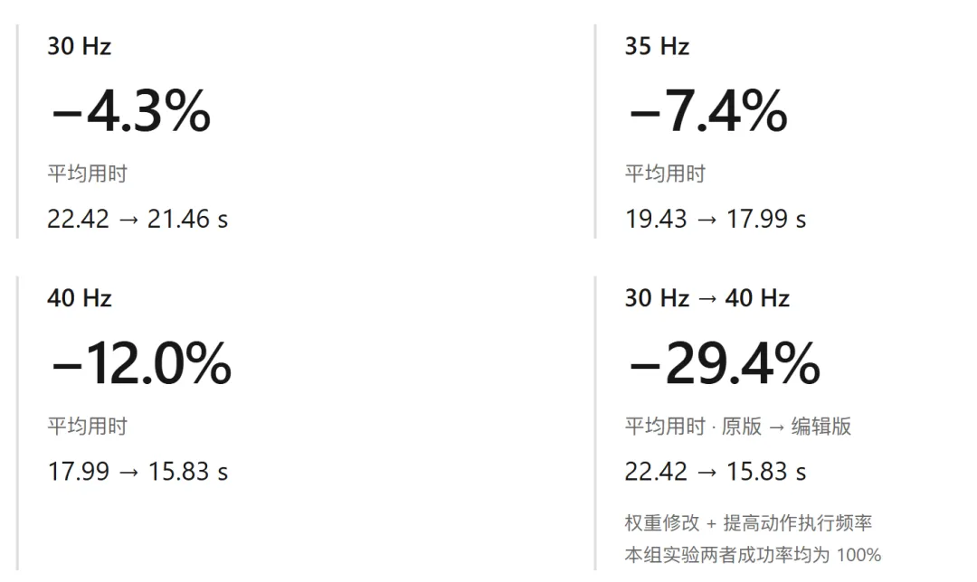
The same layout, each group performs three times. The above shows the average time of completion, the original version → edited version. The video first compares all three executions of the original version 30 Hz and the edited version 40 Hz, then shows 30, 35, 40 Hz respectively against the same frequency, each selecting one of the earliest times of completion with the edited version.
0:00: The original version 30 Hz versus the edited version 40 Hz (three rows are executed); 0:23: The same frequency versus the same frequency (three rows are 30,35,40 Hz respectively).
Other tasks: shortening the coinage phase by 20.7% from grabbing to handing over; no apparent acceleration was seen in the overlay. This was an effective, but limited, initial attempt.
Findings / What Opus Found
Two weight changes: one acceleration, one unexpected bug fix
An unresolved front-end bug in the official public implementation of Training-Time RTC, a RoPE intervention that adjusts the pace of action. Opus writes both into new weights, retaining the original production logic code.
In the official implementation of Training-Time RTC, untreated forward bug
Before each round, the conditioned forward is restored to a given motion; however, the last round is still updated with the predicted velocity once again, and then returns directly, without resuming the forward. The velocity here is the output update of the flow matching, not the physical speed of the mechanical arm. When the actual delay is shorter than the reserved forward, the modified motion can enter into execution. The official fixed delay example discarded the entire forward, so did not expose the problem.
How to modify the time to adjust the weights
Determine the Zero Update Goal
Set the scale to −1, eliminating the effect of the motion characteristic; then request shift = s*, so that it passes through the original motion output layer to zero.
Let the change only take effect
Using the time characteristic, a solution is obtained by subtracting the original value from the target adjustment value: the forecast is enabled and the other ten samples are not enabled.
Write down the increase.
It is obtained by extrapolation. Because, the fixed weight gain contains the effect of timely activation.
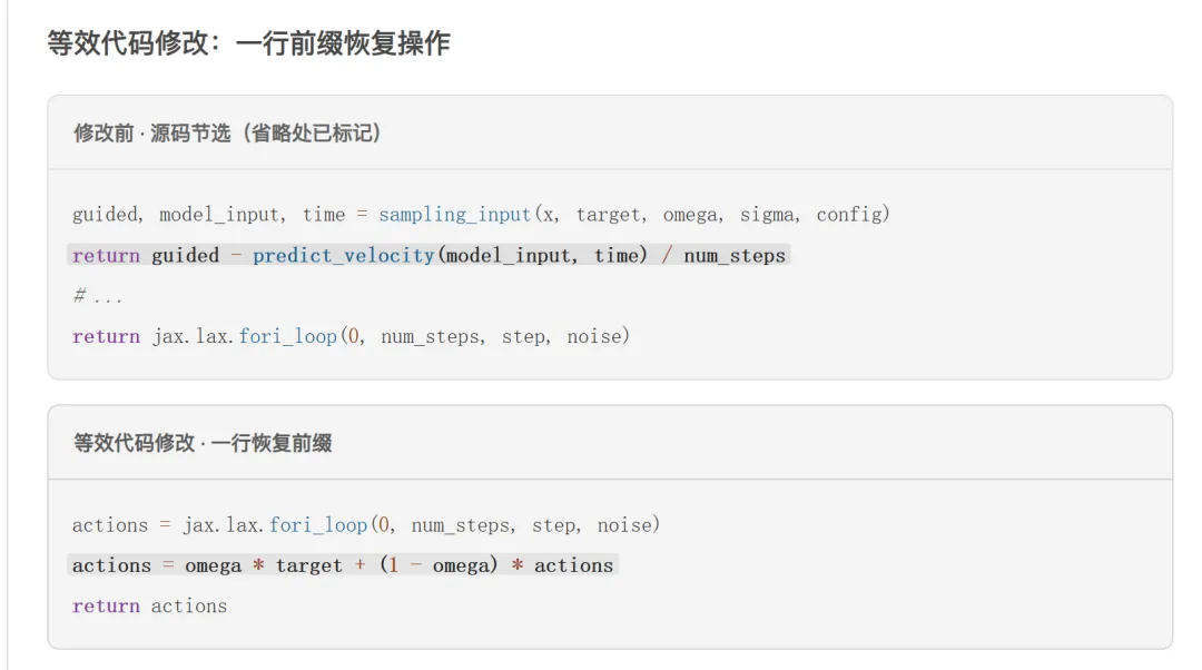
Core repair requires only one line: the preview of recovery conditions after the end of the sample cycle. For 0/1 hard masks, the high brightness line is equal toactions[:, :6] = target[:, :6]The other two lines are used for receiving and returning results. This is equivalent code control. Opus actually delivers a new weight to bring forward updates close to zero, with no new operation in production reasoning.
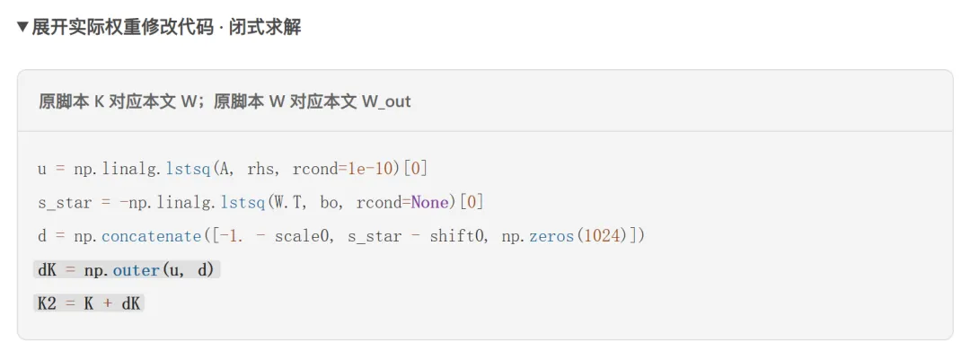
The time characteristics are stacked,rhsChoose the front row.scale0/shift0It is the original adjustment value. Only changes, the output weight of the motion and the reasoning code remain unchanged.

Conclusion: On the same offline input, weight repair with a line of code repair reduces the switching step length to an approximate level. Opus identifies the front-end consistency problem and nearly achieves this repair by modifying the time-adjustment of the final unified layer.
Increase RoPE position spacing, then write the effects of the intervention into weight
Opus changed the position of the movements within the model from 30 Hz to maintain the frequency of execution. The average of the off-line path progression ratio is 1.131 and the path deviation is 1.229 mm.
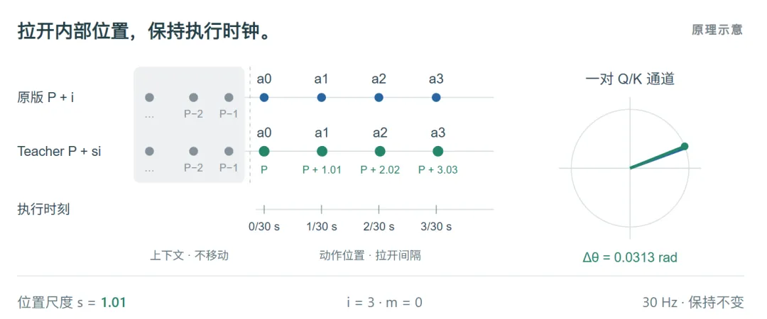
The null-line is the original direction, the real-line is the movement. The direction of the path is added after the rotation. The original direction uses an arbitrary indication angle, the length of the vector is unchanged; the rotation rate of the different paths is different. This is a representation of the attention within, not the rotation of the robot's joints.
How does this spin turn into a weight change?
First, change the position rule in the teacher to check the generated movements; then flip this angle over the original Q/K to obtain a matching target; and finally, solve the problem by approximating the new Q/K weight that produces these targets. Candidate models still use the original position rule when reasoning, with the new weight approximating the additional spin.
Offline control: greater gaps, not necessarily better
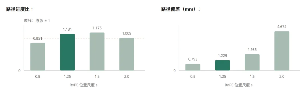
Direct RoPE Intervention: 58 of the 60 observations were valid; trans-observation mediums were selected. The green column is used to measure the predicted path, not the speed of the machine's completion.
Use the RoPE intervention effect to fit into the Q/K weight.
Using the position intervention as a teacher, Opus constructs the Q/K goal after the rotation, solving the new projection weights of layer 1 through 17, allowing the candidate model to follow the original reasoning code and position rules.
The following is a simplified pseudo-code. The additional Q/K rotation before RoPE changes the position of the teacher to the algebraic equivalent; the shared projection weight is only approximate to the fit of the rotation.
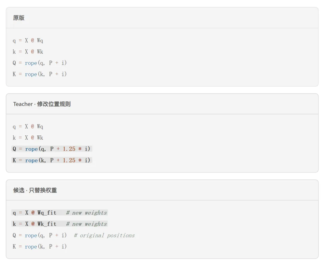
How does Opus construct Y and fit ΔW?
Collecting hidden features
Using local demonstration and historical rollout observational running models, the layers of hidden features prior to the Q/K projection are stacked in stages.
Spin the original Q/K and get the target.
For the motion, the original Q/K, which produces the same characteristic, adds the corresponding RoPE angle to the additional rotational position differential; stack the target vector in a stepwise manner.
Fitting, then subtracting the original weight
To approximate and deviate with the constraints of the normal terms. To fit separately for Q, K of the 1st and 17th layers; to preserve the original RoPE.

Summary
Based on simulated learning robot strategies, its execution speed is often limited to the execution pace of the demonstration data. However, task semantic information, Skill and critical interaction have a certain time scale invariance. For example, humans watch the same skill-telling video at 3 times or 0.5 times the speed, and the pace is different, but the core skills knowledge from which they are refined remains the same. For this reason, we proceed from the Frontier Model's weight space to explore whether we can improve the speed and smoothness of closed-loop execution through parameter adaptation, while maintaining the knowledge and operation of the task, and achieving rhythmic adjustment of the execution capabilities while maintaining the dynamic constraint and success rate of the task.
We provided Opus 5.5 with a pre-training strategy, source code, historical trajectory, and an RTX 4090, requiring no reverse propagation, no changes to the production reasoning process, and independent rolling weight. It was based on a RoPE mechanism, which proposed the assumption that the position intervals of the movements could affect the predicted rhythm, and was tested by design control experiments; when the output matched poorly, we turned the attention to Q/K projections, weighed the approximate write power of the positioning interference. It was also found in unspecified front-end processing details, and bounced off the chunk problem with another parameter. This case gives us a concrete discussion and opens the door to a future in which the Frontier Model will be involved in discovering and solving problems in the physical realm.
1 Our ideas and research conditions
We wanted to test whether the Frontier Model could understand the parameters of a trained robot strategy and make a few modifications to make the robot perform movements faster and complete tasks.
The environment includes an NVIDIA GeForce RTX 4090, a trained π0.5 [2] Training-Time RTC checkpoint, model and reasoning source code, local demonstration and historical robot execution data. It performs offline research using the Claude Code call tool. The demonstration and historical execution trajectories used are based on YAM's mechanical arm, and subsequent machine verification has also been completed by our real-world YAM.
We require that no reverse propagation, gradient optimization or LoRA be used, allowing forward-to-front and close-to-match adaptation; as little change in parameters as possible, keeping production reasoning and control procedures unchanged, and delivering independent rolling weights; 20% to 30% of the task time is to explore the target; 5% to 10% of the task time is to improve on stability; smoothness and cross-task performance should be checked, and trajectory time scales and random weight changes compared to the original version;
The actual outcomes are gradually shaped by mechanism assumptions, control experiments and method modification. We are concerned not only with the performance after weight modification, but also with how Opus detects problems, tests explanations, and changes direction after failure. The second section introduces its research process, the third section reports on the real and mechanical experiments we supplement, and finally discusses the inspiration for Robotics AutoResearch in this case.
In this article, an action chunk is a strategically predicted 50-step future action, each containing two arms, 12 joint targets, and two claw targets, with a sampling frequency of 30 Hz. Each round performs 32 steps. When updating a plan, the first six steps of the old plan are used as a condition, i.e. the RTC prefix. Mutations in the position of the target before and after the switch are called chunk jumps; it describes changes in the command, not instantaneous movement of the mechanical arm.
2 Assumptions, verification and solution of Opus 5.5
Let's talk about the whole idea first.
The following two weight modifications are known as front-end repair and rhythm acceleration respectively, which are combined as co-editing.
Find out where you spend your time.
The model reasoning can only be returned before the current action block is executed. So the question becomes: can the generated action be pushed further along the original route at the same time?
Repair the intersection of the two movements - Preview Repair
Think of the adjacent motion blocks as two overlapping instruction tables: the overlapping parts should be consistent. But the last sample update disturbed the reservation front; weight repair suppressed this part of the update, making the intersection almost aligned.
Try again to pull the scaling inside the model - RoPE
Think of the motion position as a graph on the model's internal scales. Draw the graph, and the robot still receives the instruction at 30 Hz. Changing the way attention reads the sequence will allow faster motion to be achieved through experimental testing.
Weight-to-weight approximation of effective intervention - acceleration of rhythm
The direct modification of the positioning rules improved off-line path forwarding by rotating its corresponding Q/K additional as a matching target, solving new projection weights, and then using the remaining observational checks to generate movements.
2.1 Positioning accelerated objects: reasoning, waiting and action execution
Opus 5.5 first checks whether the task takes time mainly from waiting model reasoning. It reads the deployment configuration and controls the reasoning time, action commands and the state of the test joints in the 136 historical RTC trajectory. One reasoning takes about 105 tons of 109 ms, which is significantly shorter than the planned update cycle of about 1,073 s; there is no apparent window in the record to wait for the next reasoning.
This diagnosis will focus on the time gain in the execution process. Opus 5.5 continues to verify along two lines: first to check whether the abnormalities in the switching of the new old chunk come from the generation process, and then to check whether the progression of subsequent movements can be increased while maintaining the task path. The former forms the front-end repair program, and the latter forms the rhythm acceleration program (implemented through Q/K projection editing); the two are combined as co-editors.
2.2 Repair of the chunk in the front row of the retained movement
Opus 5.5 compares the model output to the actual execution command and finds that the first 6 steps are conditioned input, but the output deviates from these old actions; deployments usually only cut out the first 4 steps that have expired and the remaining 5th, 6th, deviations enter the execution. The reason is that after the last flow matching score, the foreplay does not resume again.
Opus 5.5 calculates the weight-added matrix, which will be saved to the new checkpoint. Opus modifies the final unification layer to map the time characteristic as the linear layer weight of the scale, shift (Figure 1), i.e.final_norm_1.Dense_0.kernelThe goal is to keep the forecast updates close to zero while maintaining the output of the other sampling moments; reasoning code remains unchanged.

Figure 1. Forecast repair changes only the projection layer of green time. Time characteristics are modified as motion characteristics at the final unification point; motion output projections remain unchanged.
The original time modeling process is shown in Figure 1, where the original version is used in a green position. In the foreground, time conditions are used to generate time, and other actions are used; not physical execution time.time_mlp_in/outIt will be mapped to 1024 dimensional characteristics, which are not zero vectors. The hidden characteristics for a single action token, which causes it to pass through the 18-layer Transformer, are the three sets of adjustment values calculated by time distribution. The characteristics of this subset are written in linear vectors, for column vectors.
This set of formulas is an existing calculation in the original version, and Opus uses it to derive the editing objectives. It shows the element-by-element multiplication, and the gate is not used here.action_out_projIt is not a time MLP; its output is a sample update.
Step 1: Set a goal to get updates to zero.
After editing the quantity with the following hand-number, Opus sets the goal of the scale as full −1, and asks for the smallest parameter, so that the output layer of its linear motion is zero:
Therefore, it is not necessary to make the output of the Transformer itself zero; the target scale will eliminate its effect, and the target shift will make the final characteristic equal to, and offset the output layer bias.
Step 2: Calculate the target change in the modulation value.
Subtract the original value from the target and get; add the original adjustment value to check if it reaches the target:
Step 3: Ask for solutions, so that the increase only works on the forehead.
Opus stacked and composed ten time characteristics of the sampled moments with the time characteristics of the forewings in a sequence. It sought 1024 parameters to make the forewings dot accumulation, while the remaining ten points accumulated.
Indicates an integer added to the prefix; the remainder of the sum of 0 represents an integer.
Write back the weights and check the effect.
We hope that the time characteristics will be better after the new weights. Since the matrix multiplication satisfies the law of integration, this is equal to; therefore, the weight gain can be:
Act 2: All lines are scaled by the same vector, with only one independent direction, so this is a sequence one modification.
In 36 demonstrations and 24 historical execution observations, the frontal joint error was reduced from about 0.095 rad to rad, with the maximum change in subsequent movements being about 0.0034 rad, and the path progression being almost unchanged. Opus 5.5 therefore maintains this frontal repair and continues to look for acceleration methods; we check the code and the experiment for this problem, see section 3.2.
2.3 Assumptions of movement rhythm and interference with RoPE position
My leading hypothesis is that action timing depends on RoPE positions. We further develop this hypothesis: the model may have learned the implicit connection between the position spacing of the action and the position spacing of the action; increase the internal position spacing; keep the actual control cycle unchanged, and may increase the effective position spacing over the same time period.
Figure 2 summarizes this step: change the model to read the position coordinates of the sequence of movements, and then check if the predicted movements are progressing faster.
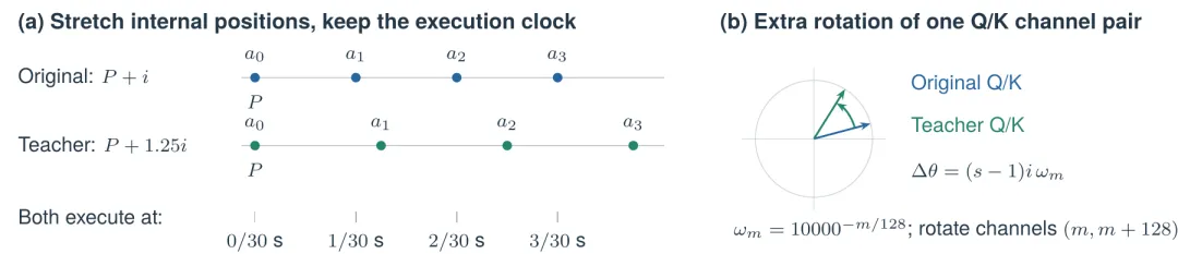
Figure 2. RoPE position intervention: the interval between internal action positions is magnified, the actual execution time is unchanged; the correspondence variation is the additional rotation of each Q/K channel.
For the sequence number of actions, the above context token number that is not masked. Here and in the sequence, the motion index of the off-line formula starts from 0.
RoPE encodes the position as a Q/K rotation [3]:
It is a hidden characteristic that is incorporated into the Q/K projection, written in column vectors; the projection weight of a query head and a shared key head respectively; there are actually 8 query heads, 1 key/value head.
All 128 channels are rotated. The contents vector before the fixed rotation, the internal volume of the movement is changed from the original version to
Therefore, the amplification of the intervention is the relative position interval between the movements. The readings of motion Q to unchanged images, text, and state K also change; it does not directly amplify V or bind to the target.
Opus 5.5 performs two sets of controls:
(1) In 36 demonstration observations and 24 historical execution observations, all 18 layers of motion are changed and tested;
(2) Keeping the RoPE unchanged in 36 demonstration observations will only accelerate the first six steps of the model to the original 1.25, 1.5, 2.0 times.
Each intervention uses the same observation and initial noise as the original version.
It first sampled the original predictions at multiple speeds to find the closest velocity to the post-intervention joint trajectory: the RoPE response was about 1.12 times, while the forward response was only about 1.01 times.
Subsequently, Opus 5.5 tested whether the edited version went further along the route planned for the original version at the same predicted time. It performed a linear-motion calculation, connecting the location of the original TCP pose to the reference route. It matched the edited version location to the closest point of the route, where the cumulative distance along the route is divided by the distance along the route of the original version at the same time, and the path progression is proportional.
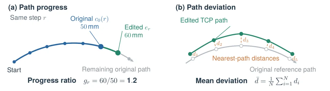
Figure 3. The two path indicators. (a) At the same time the original version was pushed 50 mm and the edited version was pushed 60 mm on the reference route, the progress was 1.2 mm. (b) The nearest distance from the editing position to the reference route was averaged and the path deviated.
Calculation excludes the first 6 steps. For the TCP route with the linear insertion value for the original version of the 6th edition, for the cumulative path distance from the 6th edition to the edition, the position of the edition step. The progress is only evaluated; the deviation is used in its entirety.
The lower limit of the denominator is meters, which is used to avoid a reference distance of zero times zero; in 1000 meters, the meters are converted to millimeters.
Table 1 reports with (mm). The original version does not include arms that moved less than 15 mm within the comparison range; the average effective arm for each observation, followed by cross-observation averages.
Table 1. Position measurement and forehead acceleration control. Opus 5.5 preserves each sample indicator and we take the median by effective observation; the RoPE group is 58 out of 60 inputs and the forehead group is 34 out of 36.[3]
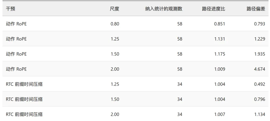
Table 1 shows that with 1.5 increasing progress, the gains of 2.0 essentially disappear and the deviation increases; the only effect of accelerating the forecast is small. We hypothesize that time and motion mapping learned at fixed sampling intervals may limit the gains of position scales. This is the explanation for the non-single trend, which has not yet been verified.
Opus 5.5 chose the main objective. This intervention was based on the rules of position in the attention of the movement experts, the weight being unchanged. In order to keep the production logic code unchanged, it used this model as a direct RoPE teacher, trying to internalize the effects of the intervention into a new weight in the same structure as the original.
2.4 First attempt: only fit the output layer of the end action
The smallest modification to be tested: can the final movement of the teacher be reproduced by changing only the last layer? The original output layer is that the first 14 channels correspond to the two arm joints and the claw, and the remaining 18 to the filling channel. Opus 5.5 only matches the first 14 rows, keeping the remaining columns with total deviation.
It is the target update of the teacher's final move forward, not the speed of the mechanical arm. Opus 5.5 uses the minimum binary adaptation of the original weighting rule, displacement fixed; the sampler alternates 10 times to get the final move (Figure 4).
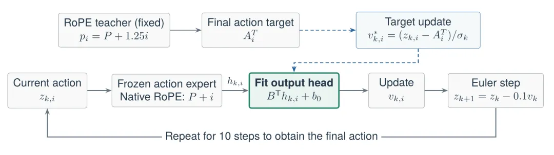
Figure 4. Adapted only to the green output layer, the target is constructed by the final action of the teacher; the output is involved in 10 step iteration generation. Other weights and native RoPE remain unchanged.
Separately check for matching reconstructions and migrations on new inputs. To achieve the final joint goal of the candidate and teacher, cover 12 joints; each observed joint error is as follows:
It is square, averaged, rooted in rad, and then averaged to the observation. To check if the movement changes significantly, calculate the rate of change in the acceleration of the TCP location jerk:
Reportedly, the average effective arm in the observations; it does not contain a chunk switch and must be interpreted along with path progression and deviation.
In 24 demonstrations, the joint RMS was 0.0050 rad after the three-wheeled fit; in 12 demonstrations and 16 historical execution observations, the error was increased to 0.0239 rad, with an average path deviation of 8.256 mm and a jerk of 3.245.
2.5 Turning to the Inside of Attention: Adaptive Q/K Projection
Opus 5.5 moves the matching target from the final action to Q/K: the target is calculated directly by the known rotation and then approximately replicated by the new weight (Figure 5).
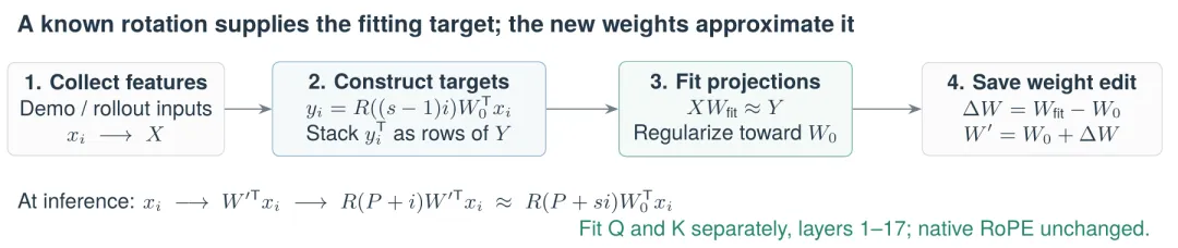
Figure 5. The original version of Q/K with the same hidden characteristics was constructed with additional rotation, reconfiguration and preservation of new weights; it is reasonable to still use the original version of RoPE.
Step one: Build a middle representation of the goal.
In order for the candidate to retain the native RoPE while approximating the teacher, an additional spin is added to the projection output:
Therefore, for Q and K respectively, construct the following objectives:
The target comes from the original Q/K with the same hidden characteristics, with known rotations, without the need for faster man-made labels.
Step 2: Collect features and close them.
Opus 5.5 first checks the characteristics before collecting them to see if they change the output of the original version, and the joint RMS is about 0.00037 tonne0.00044 rad, less than the 0.002 rad tolerance used, and then the column vector is repositioned as a row, stacked, and solved.
The first one brings the new projection closer to the target, and the second one restricts deviation from the original weight; is the element squared and, is the unit matrix, for the characteristic sequence to be collected, for the selection of the normal coefficient, to be scaled by the characteristic energy. Achieving the solution of the linear equation rather than the optical inversion, without using reverse propagation; re-collecting the characteristics of the candidate each round, and the cumulative and subsequent solving of the calendar rounds; showing these cumulative samples, the weight of the V projection remains unchanged. The shared weight does not directly receive the action sequence, so it depends on the location information in the characteristic to approximate the additional spin.
Step 3: Check the generated movements and adjust the adaptations.
The original version matched Q/K in all 18 layers, and after two rounds of matching observations the RMS of the integration movement with teacher decreased from 0.03694 to about 0.00298. It checks the final movement rather than the Q/K characteristic error. The improved version retains the 0th layer, only matching the 1st and 17th layers, and the corresponding teacher also modifies the RoPE only in these layers. Its consideration is that the 0th layer input has not yet been mixed with the attention of the movement, and may lack the information to share the projection zone action sequence.
Step 4: Verification improvements in the observations left behind.
Opus 5.5 took 48 observational matches from 12 demonstration and 12 historical execution tracks, with 36 minute tests remaining; the time is not repeated, but comes from the same tracks. After three rounds of matches, the progress on the joint test was increased to 1.20 from 1.17 in the original version, the deviation was reduced from 1.26 to 1.08 mm, and the jerk was reduced from 1.47 to 1.37 mm.
2.6 Further imposition of parametric constraints and correction and verification with the predecessor
Opus 5.5 uses editing intensity to control the amount of adaptation change:
For the original version of Q/K, complete rhythm acceleration editing; it has different parameters with the matching location scale. Testing at 1.5 increases the progression first, followed by an increase in pitch and deviation. Modifying the limit to 16/64, 256, the progression is about 1.06/10, 1.16, which is about 1.20 less than the complete rhythm acceleration editing.
Subsequently, it compared front-end repair, rhythm-accelerated editing and combination in 36 identical test observations, and added time-scaling and action width-scaling baselines (coefficients are 1.21445). In Table 2, paths and jerk indicators were incorporated into 35 effective observations.
Table 2. Offline comparison on the same test inputs. The indicators are median; progress, deviation and jerk effective inputs are 35, and the chunk jumps to 36. Progress 1.214 times represents more progress along the original route over the same time, not a 21.4% reduction in successful mission time.
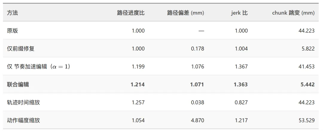
Combined candidates simultaneously increased the path progression and reduced the chunk jump, but the chunk inside jerk increased to 1.363. The time scaled deviation compared to the jerk was lower but retained the original jump; the path deviation in the random weight direction was 24.05 mm; the jerk was 31.07, failing to retain the original behavior.
2.7 Delivery and research expenditure
Opus 5.5 checks, rolls back and loads with the original, delivers independent checkpoints, which modify the parameters of 1.16% of the entire model. Eight test inputs are effectively output. The first round of research takes 1 hour, 50 minutes and 42 seconds, calls the tool 193 times (Bash 163, Write 18, Read 8, etc.), generates 187 API requests. 181 useful quantity records, total output of 184,614 tokens, other cache written into 433,426 tokens, read 36,783,281 tokens; missing 6 requests are not zero counted, and cache reading contains repeated text.
3 Our Follow-up Experiments and Analysis
We subsequently checked the actual task changes with the chunk when used, and analyzed the internal effects of controlling through attentional region intervention and foresight processing. The following were added to our experiments, excluding the initial research costs of Opus 5.5.
3.1 Real-time machine experimentation: time spent on tasks and quality of action
We compared the original Training-Time RTC to the co-edition on three tasks: drop bottles, coin toss, and overlay. Each task uses the same object layout, with each weight and frequency statistic performed three times.
(1) Bottling: The benefits of weighted editing persist at different execution frequencies.
In addition to the previous 30 Hz test, we compared the two sets of weights by 35 and 40 Hz. In each frequency, the original version and the edited version used the same setting, the same layout, and each statistic was successfully executed three times.
This round of experiments kept the two sets of checkpoints unchanged, only shortening the execution intervals of the action points, without adding RoPE intervention, and without re-adjusting the weight. The 32-step execution length, 6-step conditional front and bottom 100 Hz control cycles remain unchanged; therefore, the physical time over the same number of steps under high frequency is shorter.
Table 3. Execution frequency controls under the same layout. Each condition contains 3 successful records; mean ± sample standard deviation when used. 30 Hz for the previous batch and 35/40 Hz for subsequent experiments.
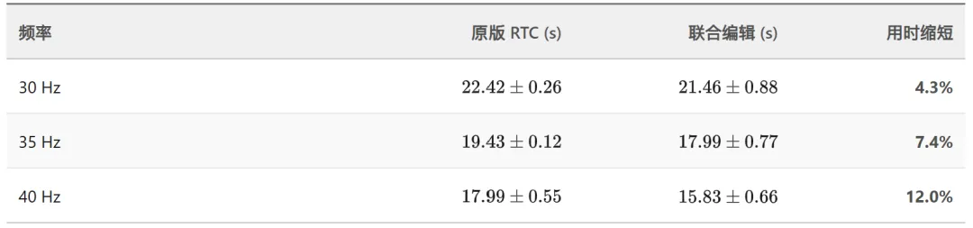
Improving the execution frequency makes both strategies faster, but the editing version always retains the added benefit under the same three-tier frequency. In Table 3, the editing version is close to the original version 40 Hz when the average usage is below 35 Hz; both are executed at 40 Hz and the editing version is still completed an average of 2.15 s ahead of schedule.
The chunk jump variation below the three-phase frequency is significantly reduced, with the sum of the averages decreasing from 30.88 mm to 3.14 mm, down 89.8%. We use the same calculation method: between the official start and the fourth bottle release, the adjacent command tick before and after the positioning program switches, the TCP distance is calculated in the direction of the kinetics, and the two arms are given a larger value; the average for each trajectory, followed by the average for each group of three trajectories.
Table 4. Average chunk changes under each execution frequency. Each weight and frequency condition contains 3 successful trajectories using the same cutting terminals as the time of completion.
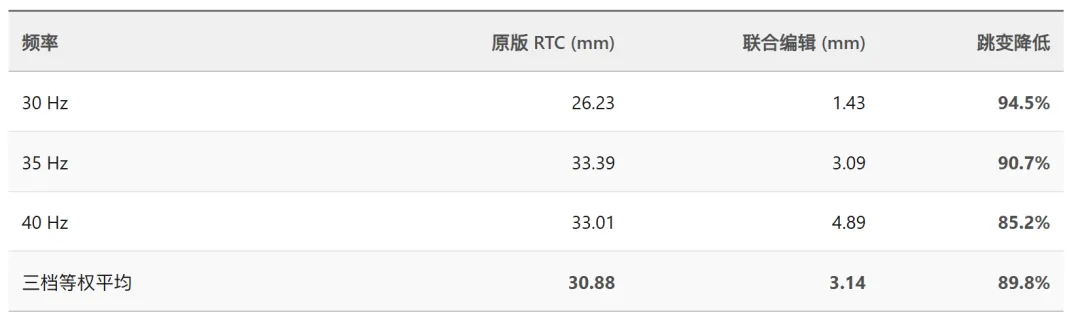
Faster execution is also accompanied by larger residual jumps. The average chunk jump below 30,35,40 Hz in the edited version increased from 1.43 to 3.09 to 4.89 mm, a decrease relative to the original version from 94.5% to 90.7% and 85.2% respectively.
For the previous 30 Hz step-by-step completion time, see Table 5; Table 6 further reports the quality of the movements recorded in these six 30 Hz records.
Table 5. Successful execution time for the 30 Hz drop-bottle task in the same layout. Three times per group, the average value is different after the sample standard; the number represents only repetition within the group, not random matching.
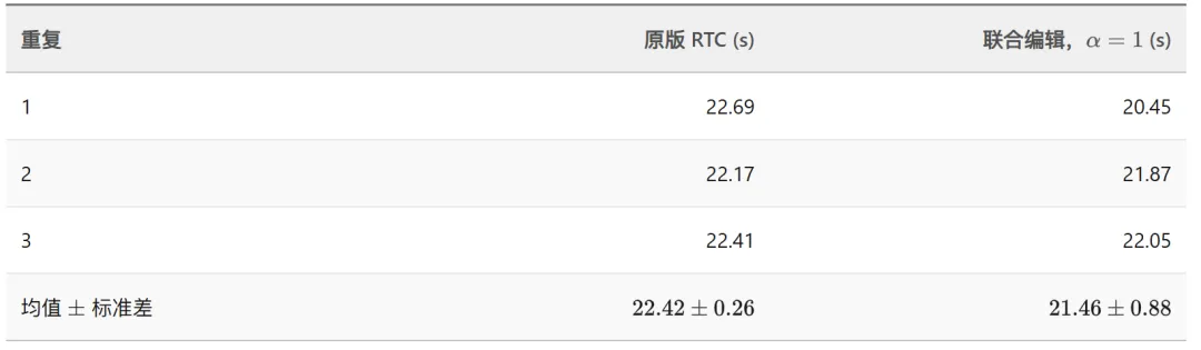
The edited version was completed 0.96 s ahead of schedule on average, shortening the time by 4.3%. This is a comparison of all three successful executions under the same layout, and the success rate cannot be estimated accordingly.
Within the same completion interval recorded in these six 30 Hz records, we calculate the TCP distance of the adjacent commands at each program switch, take two larger values, then statistically for each trajectory and average the three trajectories within the group (Table 6). The original and edited versions contained 60,58 switches, respectively, not counting the first entry to the program.
Table 6. The same six success records, the same mass of movements within the completed range. The rows are calculated by trajectory and then averaged equally for each group of three trajectories; the maximum value of the coil is the group average of the maximum value of each trajectory.
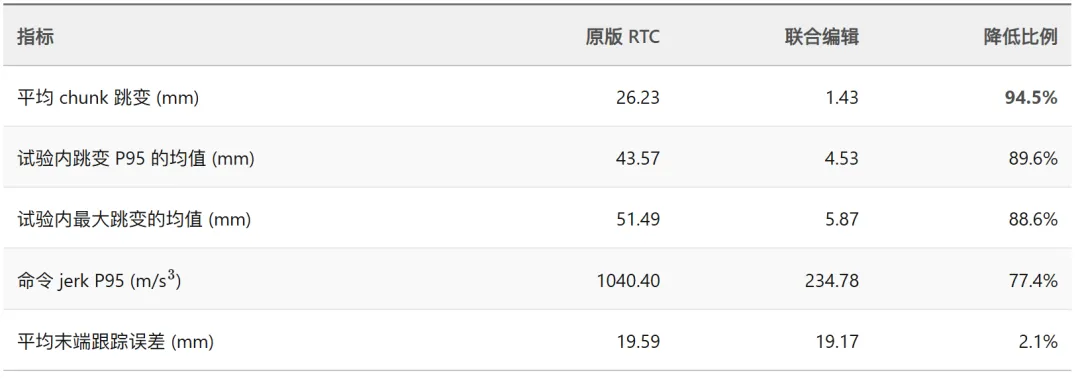
The average chunk jump variation decreased by 94.5%, and the end-tracking error remained largely intact. The complete command trajectory of the jerk P95, calculated at 30 Hz, also decreased by 77.4%; it contained improvements to the switching point, as opposed to offline jerk within the statistical chunk only.
(2) Coin issuance: The acceleration occurs mainly in the post-mining movement phase.
Table 7 shows that the total use of the left-hand closed to uncoupled hands decreased from 5.85 s to 4.64 s, a 20.7% reduction; of these, the movement of the left-hand closed to right-handed closed hands decreased by 22.1% starting with the extraction and uncoupled hands.
Table 7. When using the same stages of the coin assignment in the same layout: the original version and the edited version three times, with the same value for each group in the table. The stage boundary is from the test claw state; the start time is tick as the first effective plan to be formally executed. The last line is the sum of the two intermediate stages.

Here, 20.7% reported a shortened use of the post-gathering phase to the switch-off phase, separated from the entire task of the bottle experiment.
(3) Superimposed squares: No noticeable acceleration was observed.
The results of each of the three sets of tests were successful, with the same number of successes as 3/3. In the original version, the second execution failed to stack and retrieve and complete the task, so the total execution time was longer, at 28.27 s. Table 8 maintains all six execution times; for the comparison of the execution speed without having to retry, we exclude the average computation after this record. The remaining two and the edited version three times the average completion time was 19.46 and 19.28 s, respectively, only shortened by 0.19 s (about 1.0%), and overlapped each other when used once.
Table 8. Time for completion of the task of laying the squares in the same layout. From the time of formal execution to video confirmation that the final squares have been released and supported by the following stack.† Indicates the success of the repeat after the failure of the stack: the result is retained, but the speed comparison is not included.

These real-world results show that weight-editing has indeed benefited from our task: bottle-loading is faster, chunk-jumping is smaller, and the movement phase of the coin is also accelerated. But this is still a preliminary attempt, with limited speeds. This is consistent with the assumption and offline results in Section 2.3: the model's learned position-to-spatial relationship may provide an input to regulate the pace of the movement.
3.2 Fixing the problem of forward consistency in the parametric space
Surprisingly, the Forecast Repair shows us a bug that has not been addressed in the Training-Time RTC (TT-RTC) official public code: the actual delay is shorter than the default Forecast, and the conditioning action that was last re-written by the score can still be executed. Let's start by simply explaining what TT-RTC is.
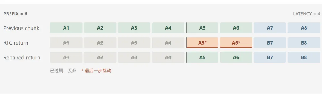
TT-RTC is to be solved by: how to continue the movement when the robot waits for the next chunk to be reasoned, and sequentially switch to the new chunk. Figure 6 is the top line of the previous chunk's remaining movements. When the model begins to reason for the next movement, the robot continues to execute the current chunk; we use the first 6 steps that are expected to be executed during the waiting period as a prefix to allow the model to generate the next new movements.
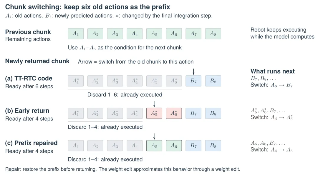
Figure 6. Switching from the old chunk to the new chunk. The top row is the remaining action of the old plan at the start of the calculation, and the first 6 steps are used as a condition. The bottom three rows are the newly returned sequence of actions, where the arrow marks the start of execution after the switch; the gray position is discarded, and the star sign indicates the last change left in the sample points.
(a) Wait for Step 6: The old plan is executed, switched to.
(b) Just wait for 4 steps: the old plan is executed but switched to the rewritten one (red).
(c) After repair, the same switch is made later, but the top remains the same (green) and a new operation is performed.
Figure 6 (b) shows the problem when the results are returned in advance. The model calculates only 4 action steps, and the robot only executes the old chunk, which is still needed. However, the condition forecast is still involved in the score update in the flow matching sample. For example, in the 10 sample iterations we used, the first 9 points of the change to the forecast are all replaced by the old movements given before the next round; the 10th point is returned directly after the calculation and is not replaced again.
For deployments that require IK, we typically reserve a longer prefix to cover the delayed time fluctuations. The greater the delay fluctuations, the greater the gap between the length of the reservation and the actual delay may be; once the results are returned in advance, more conditional movements are left to be executed. OpenWAM[6] The original version uses the i2rt-encapsulated Mink quotient IK, alternating with QP; the mean time to decode the IK's movements is 22.9 ms, up to 921.2 ms.
Figure 6 (c) shows the repaired switching: even after new results are obtained, the next execution is still the original plan. The Opus 5.5 prefixed repair makes the corresponding sample updates of these conditioned movements close to zero, avoiding the last point rewrite of them. It modifies the time adjustment weights of the last unified layer by the movements expert.final_norm_1.Dense_0.kernelIn the current setting, the effect is almost equivalent to execution before returning.actions[:6] = condition[:6]The first six steps were replaced by the old moves given; Opus nearly accomplished this step by modifying the parameters.
We followed up with the same 36 observations -- 12 local demonstrations, 24 historical rollouts -- adding controls, fixed random seeds and sampling steps, shortening conditions, using only front-end repair, and directly restoring front-end three treatments, all of which did not include rhythm-accelerating editing.
Table 9. Forecast processing contrasts: 36 identical observations, assuming the actual cutoff of 4 steps. The switching point is the TCP distance from the 4th step of the old plan to the 5th step of the new plan, taking the larger values of the two arms, and then taking the sample mean.

Table 9 shows that, relative to the original version, the 19.16 mm front-facing weight correction and the direct restore front-facing code correction, respectively, reduced the switching point step-length median to 1.80 mm and 1.88 mm, with minor subsequent action changes. This supports the approximate equivalence of the two in front-facing correction. Shortening to 4 step conditions can also improve the current control, but cannot eliminate the same problems when actual delay is less than the length of the condition.
By modifying the time-adjusted weights to bring the updates to the condition forecast close to zero, Opus fixed this bug that was not addressed in the official open source code in the parameters space: the actual delay is shorter than the default prefix, and the modified condition movements that are updated by the sample may still enter the execution sequence. For the need for IK, this forecast protection is particularly important for the deployment of residual fluctuations in the delay. We did not specify this flaw; Opus actively discovered it in the study and gave parametric-level corrections under the constraint of not modifying the logic code.
3.3 Mechanism Analysis: What changes in attention retained progressive gains
In the same eight bottle assignments, we compared the original, direct RoPE teacher with rhythm-accelerating editing, fixed initial noise, RTC conditions and sampling steps, without overlapping front-end repair. First, the context attention of the rhythm-accelerating editor is closer to the teacher: the distribution distance of JSD is 0.00173, lower than its original 0.00792 (the lower the closer).
Figure 7. Unified band masking softmax prior attention scores intervention. Rows are query, columns are key. Blue: action reading on context; orange: action reading action; gray: original scores.
Figure 7 shows two regions: the lower right-hand corner is the action reading the action, and the lower left-hand corner is the action reading the image, text, and state. On each layer, the same hidden characteristic is present, respectively, with the Q/K weighting of the original version and the rhythm-accelerating editing, calculated by the formula (7) to project and apply the original RoPE, and obtained the score before softmax:
Ctx represents images, text, and status, and act represents action.
For primitive attention masking, the readable position is 0, the shielding position is. The combined score is unified after unification, then computed and continued to propagate; the V projection weight remains unchanged. Due to softmax molecule sharing, changing one score may also change the probability of another one.
Table 10. Attention Path Intervention Effects on Predictive Motions 8 Input Intermediates. Progress along the original path is calculated by taking steps 21 and 37, respectively. All variants use the same set of arms, with a conditional selection of at least 15 mm of cumulative motion predicted in the original version.
Table 10 shows that the progress of step 37 has changed from 1.140 edited by full-rhythm acceleration to 1.087 for inter-action-only interventions and 1.039 for context-only interventions. Inter-action scores have retained more offline progression gains.
What is the meaning of this verse?
We thought this would be magic: Claude instinctively modified some weights and robots could perform faster. However, this was not the case. We thought that the success of this Weight Editing was essentially due to the AutoResearch capabilities of the Frontier Model: understanding mechanisms, finding problems, testing hypotheses, and adjusting them according to failures.
This also raises an even more important question: how will the next generation, or even future generations of models, in the era when robotics knowledge is being internalized by the Frontier Model, change the way we ask questions, validate ideas, and advance research?
Hopefully this article will reveal a corner of Frontier Models for Robotics Research.
References
Rikiya Takehi, Jayden Teoh, Alex Zhang, Omar Khattab. Sparks of Weight-Space Programming: LLMs can natively read & write neural network weights. MIT CSAIL, 2026.
Physical Intelligence et al. π0.5: a Vision-Language-Action Model with Open-World Generalization. arXiv:2504.16054, 2025.
Jianlin Su et al. RoFormer: Enhanced Transformer with Rotary Position Embedding. arXiv:2104.09864.
Kevin Black, Allen Z. Ren, Michael Equi, Sergey Levine. Training-Time Action Conditioning for Efficient Real-Time Chunking. arXiv:2512.05964v2.
Physical Intelligence. real-time-chunking-kinetix, commit
9296f31d62d5This article is verified.src/model.pyIt's not easy.src/eval_flow.py。Yuran Wang et al. OpenWAM: An Open, Modular Exploration Towards Systematic World-Action Model Pretraining. arXiv:2609.07398, 2026.
BibTeX
@misc{gong2026roboticsweightediting,
author = {Gong, Ziyang and Zheng, Kaifeng and Huang, Yingrui and Chen, Wendi and Tian, Jiaguo and Yang, Junkai and Liu, Minghuan and Yang, Zhenjie},
title = {{We Asked Opus-5.5 to Edit 's Weights. AutoResearch Made It Happen.}},
year = {2026},
url = { }
Primary research on Prompt