The first stage of the open-source model has been almost taken over by MoE, but the shift from Dense to MoE is far from just replacing FFN with multiple Experts, Routers, load balancing, and all-to-all communications across GPUs.
Hugging Face's The Ultimate MoE Training Handbook, the first two chapters of which start with a real training session, introduces how to test GPU and cluster communication performance, build training mirrors, prepare Tokenization data, and use the same data and training configuration to run the Dense baseline with the first MoE model.
One very practical design was to first establish the Dense reference baseline and then introduce the Expert. The text gives a total parameter of 6.86B, instances of MoE that each token activates about 1.22B parameters, and changes in Loss, gradient and training behavior after switching the architecture by controlling experiments.
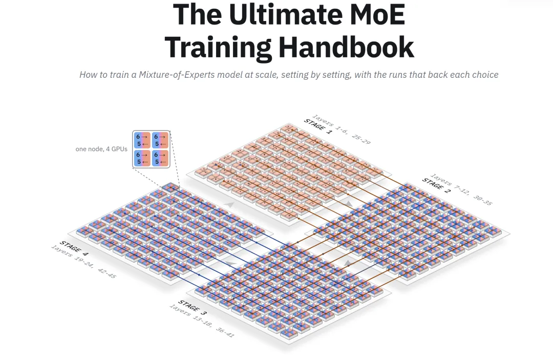
How to train a large-scale Mixture-of-Experts model from scratch: analyze the training configuration one at a time and verify each choice through practical training experiments
1. Introduction
The front-end model is in the process of becoming scarce.
It is expected to take 1 to 2 days to read this article. In order to get the best reading experience, we recommend that you do not use mobile reading.
In Artificial Analysis' Open Source Weight Model ranking, 18 of the 20 models with the highest scores used the Mixture-of-Experts (MoE) architecture. There are only two exceptions: Nanbeige 4.3-33B, ranked 12th, and Qwen 3.8 27B, ranked 13th, which use the Dense architecture.
These models also include the top-ranked models from five leading laboratories: DeepSeek V4.1 Flash 1017, GLM-5.3, MiMo-V2.6-Pro, Ling 3.1 Flash 1019, and MiniMax-M3.1-Flash.
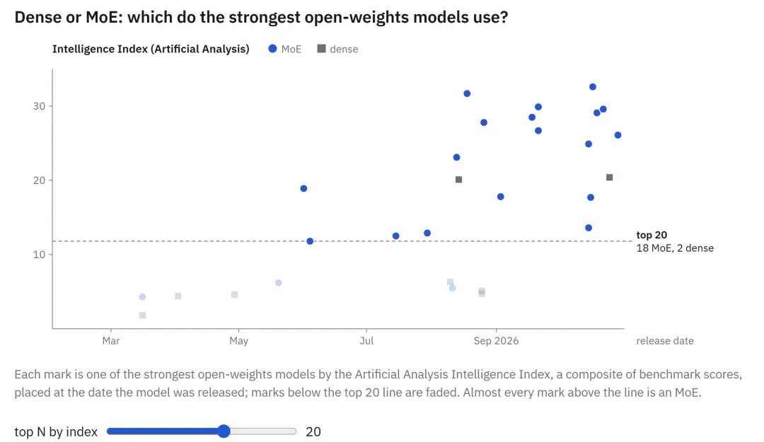
Figure 1.1
The advantage of MoE is how it allocates inference computation. Each token only needs to be passed by a few experts, so the model can accommodate far more parameters than a single token actually uses.
For example, in Chapter 2, you'll train a small MoE model. It has a total of 6.86B parameters, but the actual activation parameters for each token are only 1.22B.
The real difficulty lies in how to save the amount of computation during the reasoning phase and convert it into an improvement in training speed.
We have previously published an in-depth guide to model training, the Smol Training Playbook, which mainly introduces the training of the Dense model, but only covers part of the design of the MoE.
Since the manual's core model SmolLM3 is a Dense Transformer, its training process does not require MoE-specific technology, such as Expert Parallelism.
However, we still have a brief introduction to MoE in the Going Sparse: MoE section of the manual, covering some high-level architectural design options, including scarcity (Sparsity), granularity (Granularity), Shared Expert (Shared Experts), and load balancing (Load Balancing).
The chapter also identifies the main sources of distributed MoE training complexity: Expert placement, load balancing, and All-to-All communication, but does not elaborate on the specific implementation details.
This handbook will start from the list of issues, one by one.
From the Dense model to MoE, you have to face three new challenges:
Router: Router: Router:Decide which Expert to use for each token.
Load balancing:Ensure that the load between different Experts is balanced.
The GPU Token exchange is as follows:When the Expert is assigned to different GPUs, each layer of MoE needs to exchange tokens between these GPUs.
Each aspect introduces a new configuration that never appeared in the Dense model training, as well as a whole new way of training failure.
The following chapters will analyze these configurations one by one, discuss their specific details in depth, and provide code that can be run directly. In most cases, we will also provide direct results and data from our own clustered experiments.
A failed workout usually only tells you what the symptoms are, but it doesn't tell you directly why.
The chart below provides a high-level fault-finding guide to help you trace the roots of the problem: first, look at what went wrong in the training run, then find the first anomalous signal (i.e. Canary in the Coal Mine), and finally read the corresponding section explaining the potential causes in this article.
If you have a problem running the training, you can always refer to this chart.
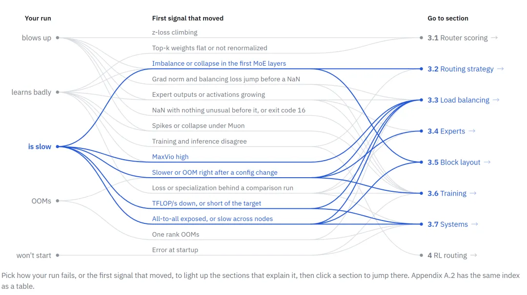
Figure 1.2
Before the official start, let's briefly explain to the readers what this manual is aimed at.
Who is this handbook for?
If you've trained a Dense model on GPU clusters and want to train a MoE next, this handbook will help you.
The second chapter introduces the necessary environment configuration and trains you to complete a small MoE model at a single node.
If you're more interested in how MoE works and what designs the current front-end model uses rather than actually running a MoE, you can jump right to Chapter 3: Anatomy of MoE Training.
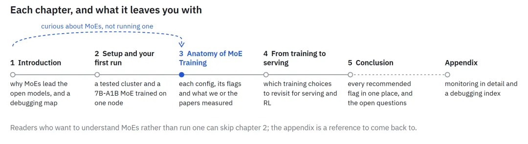
Figure 1.3
When the Expert is assigned to different GPUs, each layer of MoE needs to exchange tokens between GPUs. This is a communication model that we have never used before when we trained the Dense model.
So before you modify any of the lines of code in your model, can you be sure that the GPU connectivity links in clusters can reliably support this mode of communication?
Setup and your first run)
What do you need?
All the commands in this chapter are written for a unified machine environment to ensure a consistent operating environment for everyone: a Slurm cluster composed of eight-card nodes.
This section will discuss this environment configuration, how to use a GPU even without the GPU at all to read this article, and how to rent an eight-card node through Hugging Face Jobs. If your machine configuration is different, you can still refer to the explanation and adjust the commands according to the actual situation.
Assumptions about the cluster environment of the command
These commands require the use of a Slurm cluster, where each GPU node is equipped with eight GPUs.srunStart the task inside the specified mirror.
2.1 The nodes in Section 2.1 are ready to check using NVIDIA's DCGM diagnostics (DCGM diagnostic tool). Our experiment runs on AWS P5 nodes connected via the Elastic Fabric Adapter (EFA) and each node is equipped with eight 80 GB H100 GPUs.
Much of the content of this chapter can be done on a single node. Both the Dense baseline model and the first MoE model require only one node equipped with about eight 80 GB GPUs.
Only network checks require more nodes: All-to-All tests in section 2.1 run on two, four and eight nodes respectively; EFA mirrors in section 2.2 complete validation at two nodes.
The software environment comes from two fixed versions of source code.
The first is the NGC PyTorch mirror.26.06-py3We will import the mirror in Section 2.2 and expand the network library needed for the clusters on this basis.
The second is fixed to commit.d6316eb45Megatron's code repository. We don't build it directly into the container mirror, but we upload it when it's running.
In addition, you need a file system that can be read by both the CPU worker and the GPU node at the same time, as Section 2.3 tokenizes the data on the CPU subdivision, and training tasks require reading the processed data from that file system.
Using a GPU and not even using a GPU reading
Even if you don't have a cluster, you can still read most of this article.
The third chapter will break down the various components of the MoE Layer: what is the role of each part, how the front-end model is chosen, and what is the evidence that supports these choices. You can read this chapter from beginning to end without running any code; and then use the configuration parameters in it after you have the corresponding hardware.
Chapter 4 discusses further how these design options extend beyond pre-training, including model Serving and RL.
In this chapter, Section 2.3 tokenization runs on the CPU. It provides a small example of a single machine that can run on a single machine without the need for Slurm, so you can generate and check data files in the same format that training tasks read.
In the 2.4 and 2.5 sections of the training program, assuming you have eight GPUs of about 80 GB, the MoE model will distribute its Expert to all eight GPUs.
If you have fewer GPUs, these two sections can be used as a method reference, focusing on understanding which configurations remain unchanged in the two runs, how to select the width of the Expert, and which indicators should be compared.
The All-to-All test in Section 2.1 and the EFA environment configuration in Section 2.2 require multiple nodes to run as described in the text.
Rental nodes on Hugging Face Jobs
If you want to run a single-node experiment but don't have the same hardware, you can use Hugging Face Jobs.
It can run Docker mirrors and specify commands on Hugging Face machines and charge by the minute.
Any individual user or organization with a positive Credit Balance can use the service. Monthly quotas provided by PRO, Team or Enterprise subscriptions can also be used to pay for Jobs tasks.
hf jobs hardwareThe largest hardware configuration on the list contains eight GPUs that meet the needs of 2.4 nodes and 2.5 nodes.h200x8It is equipped with eight 141 GB H200 GPUs.
A Job is commonly defined by Docker mirrors, execution commands, and hardware configurations. Mirrors can come from Docker Hub or Hugging Face Space.
Therefore, to run the experiment in this chapter on Jobs, it is necessary to pack the mirror constructed in clause 2.2 as a Docker mirror and replace the Slurm launcher with the Jobs command.
If no other overtime is set, Job will stop after 30 minutes of running.
First, run the following command to see if Job can identify all eight GPUs:
hf jobs run --flavor h200x8 --timeout 10m \
    pytorch/pytorch:2.6.0-cuda12.4-cudnn9-devel \
    python -c "import torch; print(torch.cuda.device_count())"
Whether you're running training programs on your own cluster or renting out nodes, the actual performance of the machine won't necessarily meet the hardware specifications.
So how do we find out if a GPU or a communication link is performing less than expected?
2.1 Test your hardware
Before starting to adjust the model, it is first necessary to determine what performance the machine can actually provide.
I've been using Megatron for a long time.alltoallAt the dispatcher, each MoE Layer sends the token to the corresponding Expert's GPU and then sends the computation results back through another All-to-All communication.
Therefore, the connectivity links between the GPUs themselves need to be tested. Even if the All-Reduce test results are normal, it is not clear how quickly these tokens can be exchanged.
Before starting the training, the following checks should be run in the already allocated Job resources.
It's been a long time coming.srun --container-imageYou can start the container. The next section will discuss how to prepare the training mirror.
Check each node
First, a readiness check is performed on each node that has been assigned.
NVIDIA's DCGM offers multiple levels of diagnostic functionality. Among them, Level 1 is dedicated to ready inspection; the higher level will add more tests to help investigate hardware failures.
The following command launches a task at each node so that you can check the results of each node one by one before starting training.
NNODES=$SLURM_JOB_NUM_NODES
srun --nodes="$NNODES" --ntasks="$NNODES" --ntasks-per-node=1 \
    dcgmi diag -r 1 --fail-early
If all nodes are checked, communication testing can continue.
If a node does not pass the inspection, it should retain its diagnostic output and investigate the issue before continuing.
For example, in one of our experiments, a Level 2 diagnosis found three GPUs at a node to have temperature violations, and neither PCIe nor high-resolution tests were passed.
More time-consuming diagnostics should be arranged in a separate maintenance window.
NVIDIA defines Level 3 and Level 4 as post-diagnostic testing used by administrators, while Level 1 is used for ready-made testing.
Preparing for diagnostic imaging
If your group has already providednccl-testsThe mirror can be directly viewed through the mirror.NCCL_TESTS_IMAGESet as a corresponding path.
Otherwise, if you use an AWS cluster with EFA, you can import a public mirror maintained by the AWS NCCL test program.
Select a file system path accessible to all assigned nodes:
NCCL_TESTS_IMAGE=/shared/images/nccl-tests.sqsh
mkdir -p "$(dirname "$NCCL_TESTS_IMAGE")"
enroot import -o "$NCCL_TESTS_IMAGE" \
    'docker://public.ecr.aws#hpc-cloud/nccl-tests:latest'
The imported SquashFS file should be saved along with the baseline test results for re-importation.latestWhen labelled, a different version of the mirror may be obtained.
To ensure that the import process can be replicated, a tag with a clear version number should be selected from the AWS test program, rather than used.latest。
The AWS test program also provides Dockerfile, which can build mirrors on its own when needed.
If other network interconnection architectures are used, a combination of CUDA, NCCL, MPI and network plugins supported by the cluster should be used.
This is the first time we've seen this.nccl-testsConstruction instructions describe how to select the paths for these libraries.
Multi-node testing requests are enabled.MPI=1The following Benchmark assumes that MPI can be started through Slurm's PMIx integration, so it is necessary to ensure that the MPI configuration in the mirror matches your cluster environment.
Measuring the actual use of Collective communication performance
After all nodes are checked, all-to-all bandwidth across the entire resource allocation range can be measured.
The following command starts a Rank for each GPU and swaps a Buffer of 8 GiB between each Rank, consistent with the large message volume configuration used in our baseline testing.
It's ready to use in advance.NCCL_TESTS_IMAGEIf you're in the mirror,nccl-testsIf installed elsewhere, the executable file path needs to be adjusted accordingly.
srun --nodes="$NNODES" --ntasks="$((8 * NNODES))" \
    --ntasks-per-node=8 --gres=gpu:8 --mpi=pmix --cpu-bind=none \
    --container-image="$NCCL_TESTS_IMAGE" --no-container-mount-home \
    /opt/nccl-tests/build/alltoall_perf \
    -b 8G -e 8G -g 1 -c 1 -n 20
First, check the Rank list and then analyze the test results.
For example, a resource allocation consisting of two 8-card nodes should list 16 Ranks.
It was then checked under the corresponding test scale.busbwand#wrongTwo rows.
Below are the out-of-place results from our two node baseline tests, with other columns omitted:
size (B)      busbw (GB/s)    #wrong
8589934592    77.14           0
#wrongThe result is 0, which indicates that the test has passed the correctness check.
The bandwidth values provide a reference baseline for subsequent testing. Subsequent testing should maintain the same number of nodes, the number of GPUs per node, and the test parameters for comparison.
At the same time, a list of nodes involved in the test should be recorded, so that if a performance decline occurs afterwards, it can be traced back to the machine specifically involved.
In another separate two-node resource allocation, we set the NCCL optimization environment variable for a bandwidth of 39.84 GB/s under the same message scale as tested. Therefore, the nodes and configurations used for each test should be recorded.
All-Reduce is still a valuable control indicator, but on the same machine, there may be significant differences in the performance of the two types of collective communication.
In the two slower nodes tested above, the All-Reduce bandwidth reached 398.52 GB/s, while the All-to-All bandwidth was only 39.84 GB/s.
For MoE models that require cross-node exchange tokens, the second indicator is the one that can actually test the corresponding communication patterns.
Baseline for resource allocation of different sizes
As the number of nodes increases, the proportion of data that needs to be transmitted across node networks in all-to-all exchanges also increases.
Our multi-node test explains why it is necessary to build a baseline based on the number of nodes:
Two nodes: 77.14 GB/s
Four nodes: 39.25 GB/s
Eight nodes: 30.91 GB/s
When comparing the performance of different resource allocations, a baseline below the number of corresponding nodes should be used to ensure that the size of the message and the result column are consistent.
Prior to determining the reference baseline, the test should be repeated in a configuration that is known to run normally, while the hardware, software and test parameters are fixed.
Depending on the range of performance obtained, the new resource allocation will be judged on whether it meets the training requirements.
A practical initial strategy is to require the bandwidth to reach at least 90% of the baseline while correctly checking.
For example, for the above two node test results, the bandwidth threshold should be set at about 69 GB/s.
The specific threshold should be adjusted according to the performance fluctuations actually observed by the cluster.
For example, if the unit uses a fixed threshold of 33 GB/s, the two previously poorly performing nodes will be accepted, while the eight-node test results will be rejected.
The baseline should remain unchanged in the allocation of resources when investigating poor performance.
If you want to try an NCCL optimization environment variable, you should use the same test parameters at the same node and in different configurations.
Our previous default configurations and custom configurations used different node combinations, so the bandwidth differences between the two cannot be used to determine exactly what impact these environmental variables have.
Changes in performance during inspection training
If you want to check the hardware status regularly during training, you can use the parameters provided by Megatron:
--gpu-sniff-test-interval <n>
The parameters will be checked before the start of the training and then every second.nThe next generation is executed again.
The inspection included an all-to-all communication within the Expert Parallelism Group.
If a performance decline occurs, the system will mark Rank with an Outlier Warning that will require further investigation.
The previous diagnostic lens has helped us test the GPU and its connectivity links.
Next, we need to make sure that the trained mirrors have access to the same hardware, so we prepare the trained mirrors and check the network libraries in them.
2.2 Build your image
There are two parts of the training environment that need to be configured correctly: a library that performs GPU computing and a network library that connects different GPU nodes.
We first configure the first part of the NVIDIA PyTorch container and then add the necessary network support to the cluster.
Keeping Megatron in a separate code repository allows you to modify the training code without changing the mirror.
Here are examples using Slurm, Enroot and Pyxis.
The base lens is for NGC PyTorch.26.06-py3The network-related configuration is for the AWS P5 nodes we use with EFA.
If you are using other clusters, the network protocols supported by the cluster should be used for the part of the network.
Importing basic mirrors
Enroot will import the container mirror into the SquashFS file, after which Pyxis can pass it.srunStart the mirror.
Select an output path that can be accessed by a computational node and then import the base mirror:
IMAGE=/path/to/images/pytorch-26.06.sqsh
enroot import -o "$IMAGE" docker://nvcr.io#nvidia/pytorch:26.06-py3
Keep the Megatron code warehouse outside the mirror and mount it in the container when training starts.
The configuration parameters in this article are for commit.d6316eb45• Clearly switching to this version ensures that the code you are reading is consistent with the code actually running.
The source code description lists the version of the mirror and the code Commit used for each measurement.
Placing the code repository, along with subsequently generated data and Tokenizer, in a file system that can be read by the CPU worker and GPU nodes.
In the following order,SHARED_ROOTIt's a great way to get to know each other.PROJECT_DIRShow project directory. The supporting script will be cloned to the project directory.scripts/It's in the folder.
export SHARED_ROOT=/path/to/shared/work
export PROJECT_DIR="$SHARED_ROOT/moe-blogpost"
git clone  "$PROJECT_DIR/scripts"
git clone  "$SHARED_ROOT/Megatron-LM"
cd "$SHARED_ROOT/Megatron-LM"
git checkout d6316eb45bf1bfbb6f1f848c0b56e55166564d80
Verify the GPU access
Before adding a cluster network library, first check if the base lens is successfully imported into PyTorch and Transformer Engine, and if the GPU is recognizable.
The following commands run on a node that has been assigned eight GPUs, using the previous setup.IMAGEThe path:
srun --nodes=1 --ntasks=1 --gres=gpu:8 \
    --container-image="$IMAGE" --no-container-mount-home \
    python -c '
import torch, transformer_engine
print("torch", torch.__version__)
print("transformer_engine", transformer_engine.__version__)
print("device_count", torch.cuda.device_count())
x = torch.randn(8).cuda().sum()
print("cuda sum ok", x.item())
'
The original mirror reported the following versions and the number of devices:
The last line of the command also produces a query and result that is computed on the GPU, so it is necessary to simultaneously check whether the library input is normal and the result of this computation before continuing.
torch 2.13.0a0+8145d630e8.nv26.06
transformer_engine 2.16.0+4220403e
device_count 8
CUDA calculations are used to check that the GPU within the current node is running correctly.
If communication between different nodes is required via EFA, the following network plugins and their dependencies should be added.
Added EFA support
On our AWS nodes, the network layer is made up of EFA user statements and data.aws-ofi-ncclPlug-in composition. The plug-in needs to be built for the NCCL inside the mirror.
The version used in this build is:
EFA Installer:
1.49.0aws-ofi-nccl:v1.19.2
Both versions should be recorded together with the base lens version in the built-in configuration.
EFA mirrors build scripts to create a writeable Enroot container from the base mirrors.--skip-kmodInstall EFA user mode libraries and compile network plugins for NCCL in mirrors.
It will then export a new SquashFS mirror and remove the temporary container.
Run the script on a computing node that already has Enroot and GPU access, and specify a new output path:
EFA_IMAGE=/path/to/images/pytorch-26.06-efa.sqsh
bash "$PROJECT_DIR/scripts/build_efa_image.sh" "$IMAGE" "$EFA_IMAGE"
After the start of the training, there will be an increase in the number of participants.EFA_IMAGEUsed--container-imageThe path.
The script is responsible for preparing the network layer. The following environmental variable configurations need to be used in conjunction with the mirror to ensure that Job can find and select the correct network library.
The library path here points to a copy of the library installed inside the container.NCCL_NET_PLUGIN=ofiThe name of the plug-in is selected.
In our environment, if the file system path is entered directly as a plug-in value, NCCL creates an invalid library name.
export LD_LIBRARY_PATH=/opt/amazon/ofi-nccl/lib:/opt/amazon/efa/lib:${LD_LIBRARY_PATH:-}
export NCCL_NET_PLUGIN=ofi
export FI_PROVIDER=efa
export FI_EFA_USE_DEVICE_RDMA=1
export NCCL_SOCKET_IFNAME='^lo,docker0,veth_def_agent'
export NCCL_DEBUG=INFO
Socket Interface Exclusion configuration is aimed at the initial connection used by the NCCL to establish communication.
On our nodes, the NCCL has chosenveth_def_agentIn the end, the link to the link-local address was removed and the link-local address was removed.Connection refusedIt's wrong.
After removing the interface, training tasks can be started normally.
If this configuration is to be replicated in other clusters, the list must be excluded based on actual network interface adjustments.
Verify network paths
When starting a multi-node training task for the first time, the NCCL initialization log should be checked and the training performance analyzed.
This step is used to validate the network path used by the train mirror itself.
For the EFA mirrors described in this article, it is important to look at the following log:
NCCL INFO Using network Libfabric
If you look at it,Using network SocketIt is necessary to check the plug-in loading logs close to the top.
The invalidity of the plug-in name or the lack of a corresponding version of the library may cause the NCCL to return to Socket communication.
For example,EFA_1.4The error indicates that there is no corresponding version of the library and that the problem needs to be addressed first and then tried again.
The log can confirm which transmission method Job ultimately chose, but the actual bandwidth still needs to be measured separately.
The training mirror and network configuration shall be recorded together with the diagnostic results in Section 2.1 and a clear distinction shall be made between the two test environments in order to compare their performance.
After the hardware checks and the mirrors are ready, you can start training for the first time.
The whole process starts with data: converting the original text into a token sequence and storing it in the format required by Megatron.
2.3 Tokenization (data Tokenization)
Megatron reads the training text from a pair of index files..binA token ID is stored in the file, and a token ID is stored in the file..idxThe files record the starting and ending locations of each sequence.
Prepare these documents in advance so that both Dense and MoE can read exactly the same token during training sessions, ensuring that the training data does not change at the same time as the model architecture changes.
We will use the FineWeb-Edu data set and the Llama 3.2 Tokenizer.MegatronDocumentTokenizerYou can write the required file format directly to Megatron. The rest of the job is to select the output directory, check a small sample, and then submit the complete Tokenization task.
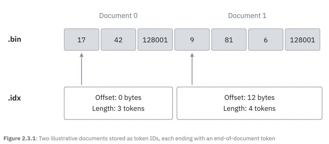
Figure 2.3.1:Two example documents are stored as token IDs, with each document ending with a token.
Get ready for Tokenizer
Keeping the data and TokenizerSHARED_ROOTBelow is the shared directory configured in Section 2.2.
Tokenization scripts run a small sample locally and then submit a Slurm Array Job to complete the task.
export TOKENIZER_DIR="$SHARED_ROOT/tokenizer"
python3.11 -m venv "$SHARED_ROOT/tokenize-venv"
source "$SHARED_ROOT/tokenize-venv/bin/activate"
python -m pip install \
    'datatrove @ git+ \
    pyarrow tokenizers huggingface_hub
The original Tokenizer warehouse.meta-llama/Llama-3.2-1BAccess authorization must be approved.
If your account has access permissions, it can run.hf auth loginAnd then use the warehouse in the download command.
Otherwise, copies can be used without authorized access.unsloth/Llama-3.2-1BThe results of our comparison show that both have the same vocabulary and token ID.
Regardless of which version is used, Tokenization and the training phase will read the same Tokenizer file that has already been downloaded.
TOKENIZER_REPO=unsloth/Llama-3.2-1B
hf download "$TOKENIZER_REPO" \
    --include 'tokenizer*' --include 'special_tokens_map.json' --include 'config.json' \
    --local-dir "$TOKENIZER_DIR"
Datatrove will read from the directory.tokenizer.jsonIt's a great way to get to the end of each document.<|end_of_text|>。
In the meantime, the Megatron has been approved.--tokenizer-modelTo receive the directory and read the Tokenizer configuration in it.
Check out a small piece of data
Before submitting a complete task, a small sample on the CPU computing node is Tokenized.
The following commands read up to 1,000 documents and retain all documents. Enter and write a separate directory to avoid mistaking the sample as formal training material.
python "$PROJECT_DIR/scripts/tokenize_first_run.py" \
    --tokenizer "$TOKENIZER_DIR/tokenizer.json" \
    --output "$SHARED_ROOT/data-smoke" --limit 1000
The forefront of exporting documents is:fineweb-edu_00000_tokens。
Next, use a training mirror prepared for section 2.2 to examine the file through the Megatron autonomous reader. You need to apply for a resource allocation that can start the container via Pyxis.
First of all, stop using the Tokenization environment to avoid interpreters in which the Python environment covers the mirror itself.
If you use an EFA environment, you'll be able to use the EFA environment.TRAIN_IMAGESet to:EFA_IMAGEIf other clusters are used, set as ready-to-train mirrors.
deactivate
export TRAIN_IMAGE="$EFA_IMAGE"
export MEGATRON_PATH="$SHARED_ROOT/Megatron-LM"
srun --nodes=1 --ntasks=1 \
    --container-image="$TRAIN_IMAGE" \
    --container-mounts="$SHARED_ROOT:$SHARED_ROOT" \
    --container-workdir="$MEGATRON_PATH" --no-container-mount-home \
    env PYTHONPATH="$MEGATRON_PATH" python -c '
import sys
from megatron.core.datasets.indexed_dataset import IndexedDataset
data = IndexedDataset(sys.argv[1])
assert len(data) > 0
print("sequences", len(data))
for i in range(min(3, len(data))):
    tokens = data[i]
    assert len(tokens) and tokens[-1] == 128001
    print("length", len(tokens), "last token", int(tokens[-1]))
' "$SHARED_ROOT/data-smoke/fineweb-edu_00000_tokens"
You should see a non-zero sequence number, and the last token of each sequence checked is128001。
This end token is the document border marker we asked Tokenizer to add.
Read the data snippet with Megatron to verify if Megatron can correctly parse the index file and read the previous sequences in the token file before GPU training begins.
Submitting Tokenization Mission
Small sample checks are file formats, while the complete task is to prepare a content that can be used repeatedly as the training experiment expands.
Submit tasks at the login node and keep the same virtual environment active.
I'm going toCPU_PARTITIONThe CPU partition is set to be clustered; if requested by the router, it needs to be added.--qos。
The script requests 12 CPUs and 24 GB of memory for each task, and requires that these workers access the virtual environment through the same path.
source "$SHARED_ROOT/tokenize-venv/bin/activate"
export OUT_DIR="$SHARED_ROOT/data/fineweb-edu"
CPU_PARTITION=your_cpu_partition
python "$PROJECT_DIR/scripts/tokenize_first_run.py" \
    --tokenizer "$TOKENIZER_DIR/tokenizer.json" --output "$OUT_DIR" \
    --tasks 100 --limit -1 --sample-rate 0.074 --partition "$CPU_PARTITION"
Datatrove will output the job ID of the assigned task.
Use this ID to pass.squeue -j <job-id>Tracking and checking the implementation of Array Job$OUT_DIR/logsFollow the log of the failed mission, and then re-submit the same command.
Each task reads a portion of the input file and randomly retains 7.4% of it before Tokenization.
Due to the different lengths of different documents, this sampling ratio does not determine the number of tokens that are ultimately output.
If the interrupted task needs to be restarted, the number of tasks, sampling rates and output directories should remain unchanged.
Datatrove will use the completion mark in the log directory to skip completed tasks.
Slices of data are transmitted to Megatron
After the Array Job is complete, it is reproduced as a list of training data.
The following check verifies the completion markings of all 100 tasks and the existence of the expected data fragment file, and then writes the prefixes for each data fragment.data-args.txtOne at a time.
Every forward responds at the same time..binand.idxThe two documents, therefore, should not be included separately in the Manifesto..binOr.idxIt's the back.
export DATA_ARGS="$OUT_DIR/data-args.txt"
python - <<'PY'
import os
from pathlib import Path
root = Path(os.environ["OUT_DIR"])
prefixes = [root / f"fineweb-edu_{rank:05d}_tokens" for rank in range(100)]
for rank, prefix in enumerate(prefixes):
    assert (root / "logs/completions" / f"{rank:05d}").is_file(), rank
    for suffix in (".bin", ".idx"):
        path = Path(str(prefix) + suffix)
        assert path.is_file() and path.stat().st_size > 0, path
Path(os.environ["DATA_ARGS"]).write_text("\n".join(map(str, prefixes)) + "\n")
print(f"wrote {len(prefixes)} prefixes")
PY
deactivate
The training will pass.--data-args-pathRead this document.
The list of data provided by this parameter is as follows:--data-pathSimilar, but avoided writing a large number of data fragment paths directly in the startup command.
The start-up script will also pass.--data-cache-pathSpecifies a perpetuated directory for storing Megatron's sample indexes. Thus, training tasks using the same dataset configuration can be repeated using these indexes.
In the initial training experiments, we used--split 100,0,0All data will be allocated to the training set.
A separate Held-out dataset should be reserved before using the training results to compare model quality.
Now that we have a regularly readable dataset and a Manifest that points to individual data chunks, we can start the Dense baseline model.
Prior to introducing Expert, a reference baseline was created using its Loss, gradient parameters and Step Time.
2.4 Dense baseline model (Dense baseline)
When an accidental event occurs in the MoE model, the Dense model can provide a specific contrast object.
Both models will use the same data, batch size and optimizer, so when Loss occurs or a training step slows down, we can first compare it to the simpler Dense model.
This baseline experiment can also be used before the introduction of the Router, as well as to verify that the trained mirror and Data Loader are working properly.
The model comprises 16 Transformer Lays, with a Hidden Size of 2,048, and a width of 8,192 for the Feed-Forward Network.
Using a word list containing 128,256 tokens, the total parameters of the model are about 1.22B.
The training program is aimed at a node equipped with eight GPUs, each with about 80 GB of storage.
Subsequent MoE experiments will repeat the same start-up script.
Start training at individual nodes
We will use Trackio to record training indicators.
Trackio is a lightweight open-source experiment tracking tool introduced by Hugging Face. Its API is similar to that of wandb, so existing code usually only needs to be tracked.wandbIt was replaced by:trackioThat's right.
Experimental data is recorded in a local database controlled by you. You can browse the results of the experiments through the local Dashboard, or synchronize the data to Hugging Face Space, and share training curves with team members in real time, with no account or paid subscription.
First, create a Python environment in shared storage. This environment needs to be created inside a trained mirror to inherit the GPU library in the mirror, and then install a fixed version of the experiment tracking tool:
srun --nodes=1 --ntasks=1 \
    --container-image="$TRAIN_IMAGE" \
    --container-mounts="$SHARED_ROOT:$SHARED_ROOT" --no-container-mount-home \
    bash -c 'python -m venv --system-site-packages "$1/train-venv" &&
        "$1/train-venv/bin/python" -m pip install "trackio==0.42.0"' _ "$SHARED_ROOT"
export TRACKIO_PROJECT=moe-first-run
Start the script using Trackio's input and send Megatron's metric indicator to each Job's corresponding independent experiment run record.
The two experiments run on the shared Project, where the data is stored.$SHARED_ROOT/trackioDown there.
The adapter uses Megatron's existing metric log recording interfaces, hence, such as:--log-memory-to-tensorboardParameters like this can still control which indicators are sent to Trackio.
For the first time, the training script will organize the training parameters into Bash mathematics.
It will use training mirrors prepared for the previous chapter, a fixed version of the Megatron code repository, a Tokenizer directory and a data manifest.
Make sure that the mounting paths are located.SHARED_ROOTdown, and willTRAIN_IMAGESet to a ready-made SquashFS mirror.
In the shared Blog code repository directory, submit the Dense task to the GPU partition.
When submitting a task, retain the environmental variables that have been extracted in Section 2.3.
The script will record the mirror path, the Megatron Commit and the data Manifest together into the output.
cd "$PROJECT_DIR"
GPU_PARTITION=your_gpu_partition
sbatch --partition="$GPU_PARTITION" scripts/first_run.sbatch dense
Slurm will reserve an eight-card node for the task.
Within the nodes, asrunThe mission will start.torchrunThe latter initiates a training process for each GPU.
I'm going to be able to run the output.$SHARED_ROOT/runs/dense-<job-id>The training log is located in the submission directory below.first-run-<job-id>.out。
This initial training run will stop after 120 iterations.
In this environment-checking experiment, both Checkpoint saving and Validation were disabled.
Before entering the MoE experiment, the running log and Trackio data should be retained, which will serve as a reference basis for the next section.
If you want to check the training curve, you can install it on a machine that can read the saved directories.trackio==0.42.0And then you start the Dashboard.
In Project, select Dense and MoE to run twice to compare them.
TRACKIO_DIR="$SHARED_ROOT/trackio" trackio show --project "$TRACKIO_PROJECT"
Understanding Training Configuration
Since both Tensor Parallelism and Pipeline Parallelism are set to 1, each GPU retains a complete copy of the Dense model.
Data Parallelism allocated Batch to eight GPUs, while both experiments enabled Distributed Optimizer and communication overlapping.
--tensor-model-parallel-size 1 --pipeline-model-parallel-size 1
--expert-model-parallel-size 1 --context-parallel-size 1
--use-distributed-optimizer --overlap-grad-reduce --overlap-param-gather
--micro-batch-size 8 --global-batch-size 512
Each micro-batch contains eight sequences on each GPU.
Eight GPUs together process 64 sequences per Micro-batch; after accumulating eight gradients, they form a Global Batch Size of 512.
When the sequence length is 4,096, the number of tokens consumed by each Optimizer Step is 2,097,152.
Keeping these values unchanged allows the step time of Dense and MoE to be directly comparable.
Learning rates are based on the Warmup, Stable and Decay three-phase scheduling strategies.--lr-decay-style WSDIt's specified.
The first step is to increase the rate of learning.5e-4The Token Budget, which was last configured, began to decline near the end.
This 120-generation run will end at Stable; training stop conditions will not reduce the learning rate scheduling schedule.
Complete Activation Recomputation enables the initial configuration to accommodate the cache budget of the baseline experiment.
In the case of Micro-batch Size 8, where native Cross-Entropy is used, if Recomputation is not enabled, the Loss computation phase will result in a cache overflow.
We retained Recomputation in both models to avoid introducing both structural changes to the model and storage optimization changes at the same time as the first comparison.
--recompute-granularity full --recompute-method uniform --recompute-num-layers 1
--cross-entropy-loss-fusion --cross-entropy-fusion-impl native
The Loss, gradient parameters and Step Time of the Dense model are stored in Trackio as a subsequent reference baseline.
When you replace the Feed-Forward Layer with Expert, these metrics will help you observe the impact of structural changes on the training process.
2.5 First training of MoE
The Dense model uses the same Feed-Forward Network (FFN) for each token. In the MoE, the router selects eight of the 64 smaller Expert tokens for each token, enabling the model to accommodate far more parameters than a single token actually uses.
We chose the width of the Expert so that the Feed-Forward parameters contained in the eight Expert tokens selected are exactly the same as the Dense Layer that replaced them.
In the end, a total parameter of 6.86B was obtained, with each token activating a model parameter of about 1.22B.
Additional model capacity also brings new costs: tokens must be sent to the selected Expert location, and Expert's output must be returned to the process that requires them.
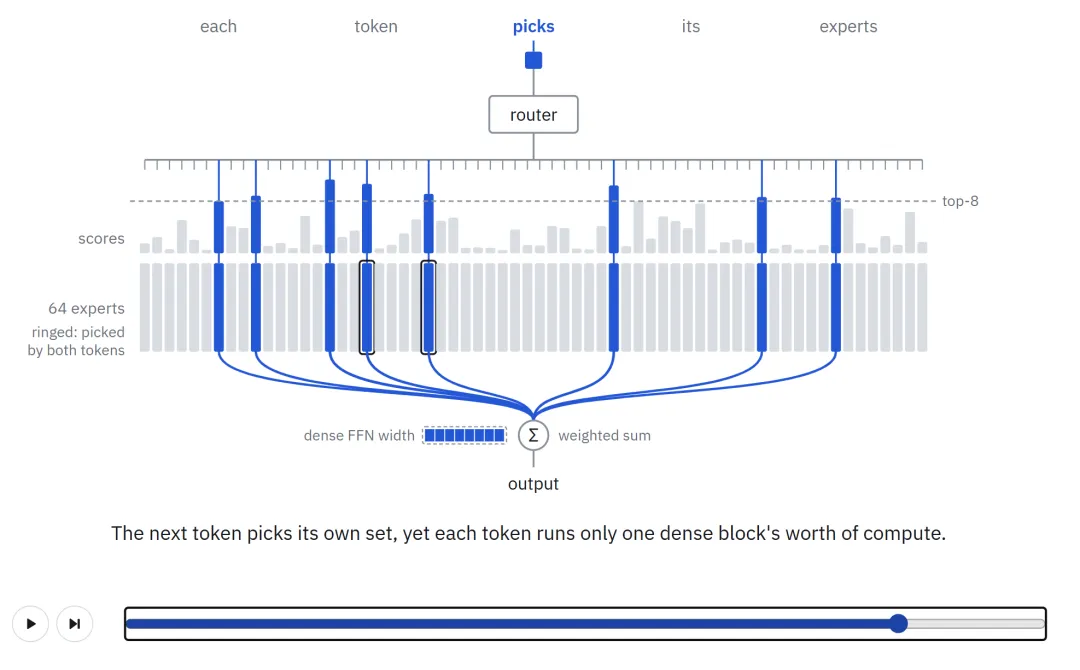
Figure 2.5.1
Replacing Feed-Forward Layer
When the start-up script is receivedmoeIn the parameters, the MoE configuration is selected.
Using the same environmental variables and GPU subdivision assignments as the Dense experiment, while keeping the mirror, code repository, Tokenizer, and data manifest unchanged:
sbatch --partition="$GPU_PARTITION" scripts/first_run.sbatch moe
Expert Parallelism increases from 1 to 8, distributing 64 Experts across eight GPUs at the nodes.
Each GPU saves 8 Expert, while the Router chooses 8 for each token from all 64 Expert.
--expert-model-parallel-size 8 --expert-tensor-parallel-size 1
--num-experts 64 --moe-ffn-hidden-size 1024 --moe-router-topk 8
--moe-token-dispatcher-type alltoall --moe-grouped-gemm
--moe-router-load-balancing-type aux_loss --moe-aux-loss-coeff 1e-3
--moe-router-dtype fp32 --moe-per-layer-logging
alltoallGrouped GEMM is responsible for the routing of tokens between different GPUs, while Grouped GEMM is responsible for the matrix multiplication of local Expert.
Auxiliary Loss encourages routers to allocate computational loads to different experts, whose coefficients are set to:1e-3。
In addition, we used fp32 to calculate Router Logits and enable layer-by-layer logging. These configurations and measurement results constitute the initial setup and reference data for in-depth analysis in Chapter 3.
All other configurations remain public, including the full Activation Recomputation.
It is important to note that the Dense model is very similar to the Dense model.--ffn-hidden-size 8192It's still in the script, and it's still in the script.--moe-ffn-hidden-size 1024It is used to specify the width of each Expert.
Calculation of activated parameters and total parameters
A SwiGLU Expert without Bias contains three weight matrices.
When Hidden Size is 2,048 and Expert Width is 1,024 the sum of the parameters of these three matrices is:
Therefore, the actual feed-forward parameters used when each token selects eight experts are:
This is exactly the same as the Dense Layer parameter that was replaced:
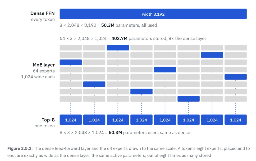
Figure 2.5.2: The Dense Feed-Forward Layer is drawn in the same proportion as the 64 Expert. Connecting the eight Expert endpoints of a token selection is exactly the same width as the original Dense Layer: both have the same activation parameters, while the parameters stored in MoE are eight times the Dense Layer.
The total of 64 Expert parameters is eight times the original Dense Feed-Forward Layer.
However, the multiplier growth of the parameters of the entire model will be smaller, as the size of Attention, Embedding and other non-Expert parameters will remain the same, and a smaller Router matrix will be added to each layer.
Adding all of the components in the 16 layers together, you get:
MoE total parameter: 6.86B
MoE is the activation parameter for each token:1.221B
The Dense model has total parameters:1.219B
Eventually, the total parameter of MoE was about 5.6 times that of the Dense model, but the activation parameters of the two were almost the same.
However, activating the same parameters does not mean the same amount of time for each step of training: distributing tokens to different experts changes how the GPU is organized, while introducing additional communication costs.
Keep the Dense reference baseline
A MoE with only a single Expert, using Top-1 Routing, performs the same function as the Dense model from which it is derived, so it should theoretically perform the same training behavior.
In our experiment, a single Expert MoE converted from Dense Checkpoint continued training in parallel with the Dense model. In 15 coordinated training steps, the Loss difference between the two was always controlled within 0.00087.
This comparison would not make much sense if MoE were to be trained from an independent initialization, as the Loss of the two runs in the fourth generation was already 2.72.
The MoE side also recorded a load balance Loss of exactly 1, along with some 32,770 gradient-zero parameters; by comparison, the Dense model has only a maximum of 17 gradient-zero parameters.
These zero gradients are derived from the Router Weight: When there is only one Expert, the Router Weight cannot obtain a gradient.
This consistency verification experiment uses Dense Checkpoint Upcycling. This conversion pathway is discussed again in Section 3.6 of Chapter III.
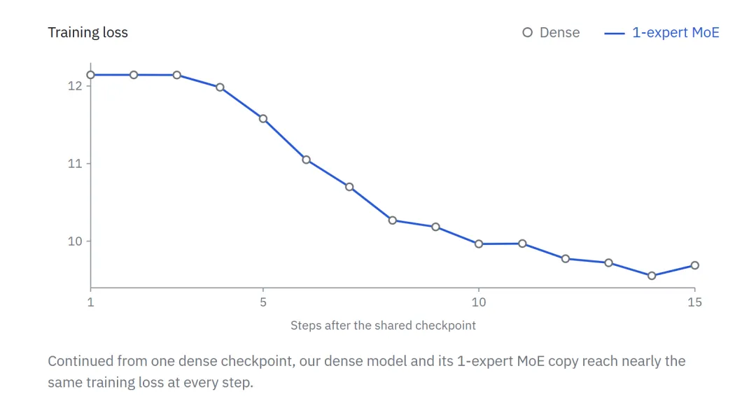
Figure 2.5.3
Under the current fixed code Commit, this Upcycling path has only been modified locally at two locations.training.pyIt's going to work.
The first amendment concerns the keyword parameters used when passing the Dense model to the Checkpoint Loader.
The current code passes the Dense model through keywords.modelCheckpoint Loader is installed, butload_checkpointThe function actually names this parameter asddp_model。
The second is the modification of the Dense model that involves loading.
The upcycling code will be updated.argsIt switches to the shape configuration of the Dense model, but the model builder reads the model configuration that was saved at launch. Therefore, the actual built-out model still retains the layout of the MoE Layer, which is ultimately missing during loading.pre_mlp_layernormThe key is to fail.
Deterministic mode allows repetitive training to be performed, making the difference between the two operations meaningful.
In the current Fixed Code Commit, enabled--deterministic-modeThe following requirements are met:
Cross-Entropy Loss Fusion must be shut down.
The TP Communication Overlap must be turned off.
The Fused Auxiliary Loss Kernel must be turned off.
NVTE_ALLOW_NONDETERMINISTIC_ALGOIt can only be set to0。
If the following environment variables have not yet been set, Deterministic Mode will automatically set:
NCCL_ALGO=RingNCCL_EP_HT_EM_AG_SCAN_MODE=1NVTE_ALLOW_NONDETERMINISTIC_ALGO=0CUBLAS_WORKSPACE_CONFIG=:4096:8
The start script for Section 2.4 is injected.--cross-entropy-loss-fusionAnd it will.NVTE_ALLOW_NONDETERMINISTIC_ALGO=1Exports are environmental variables, so these two settings must be removed before adding Deterministic Mode.
In these configurations, we reduced the Micro-batch Size of the MoE to 2, the Global Batch Size to 64, and ran 12 iterations.
The results show that the two LM Loss, Load-balancing Loss, Grad Norm and Gradient Zeros running in each generation are completely consistent.
If these determination settings are not enabled, from the first iteration, LM Loss will result in a difference of 0.00063.
Therefore, Deterministic Mode should be enabled before running or evaluating the NaN problem in two training sessions.
In the development of MoE, the Dense model and its configuration were always retained as a reference basis.
Whenever a modification leads to a decrease in training speed, or Loss does not improve, it should return to the Dense experiment in Trackio and compare Step Time, Loss and Gradient Norm under the same Batch Size and Sequence Length.
If a problem occurs in both runs of Dense and MoE at the same time, the problem is more likely to come from the training environment or configuration they share.
If the problem occurs only in MoE, there is reason to investigate Routing and Expert Execution further.
Figure 2.5.4: Using synthetic Dense and MoE training runs data showing Trackio interfaces. These curves are only used to describe interface functionality and do not represent actual measured training performance.
The Dense Reference Baseline can help you decide where to start.
Chapter 3 will break down the various components of the MoE Layer and introduce the measurement metrics required to understand its operational behavior.